Previously I presented the Kafka abstraction funnel and how it provides a simple yet powerful tool for writing applications that use Apache Kafka. In this post I will show how these abstractions also provide a straightforward means of interfacing with Kafka Connect, so that applications that use Kafka Streams and KSQL can easily integrate with external systems like MySQL, Elasticsearch, and others.
This is a somewhat lengthy post, so feel free to skip to the summary below.
Twins Separated at Birth?
Normally when using Kafka Connect, one would launch a cluster of Connect workers to run a combination of source connectors, that pull data from an external system into Kafka, and sink connectors, that push data from Kafka to an external system. Once the data is in Kafka, one could then use Kafka Streams or KSQL to perform stream processing on the data.
Let’s take a look at two of the primary abstractions in Kafka Connect, the SourceTask and the SinkTask. The heart of the SourceTask class is the poll() method, which returns data from the external system.
/**
 * SourceTask is a Task that pulls records from another system for
 * storage in Kafka.
 */
public abstract class SourceTask implements Task {
    ...

    public abstract void start(Map<String, String> props);

    public abstract List<SourceRecord> poll()
        throws InterruptedException;

    public abstract void stop();

    ...
}
Likewise, the heart of the SinkTask is the put(Collection<SinkRecord> records) method, which sends data to the external system.
/**
 * SinkTask is a Task that takes records loaded from Kafka and
 * sends them to another system.
 */
public abstract class SinkTask implements Task {
    ...

    public abstract void start(Map<String, String> props);

    public abstract void put(Collection<SinkRecord> records);

    public void flush(
        Map<TopicPartition, OffsetAndMetadata> currentOffsets) {
    }

    public abstract void stop();

    ...
}
Do those Kafka Connect classes remind of us anything in the Kafka abstraction funnel? Yes, indeed, the Consumer and Producer interfaces. Here is the Consumer:
/**
 * A client that consumes records from a Kafka cluster.
 */
public interface Consumer<K, V> extends Closeable {
    ...

    public void subscribe(
        Pattern pattern, ConsumerRebalanceListener callback);

    public ConsumerRecords<K, V> poll(long timeout);

    public void unsubscribe();

    public void close();

    ...
}
And here is the Producer:
/**
 * A Kafka client that publishes records to the Kafka cluster.
 */
public interface Producer<K, V> extends Closeable {
     ...

    Future<RecordMetadata> send(
        ProducerRecord<K, V> record, Callback callback);

    void flush();

    void close();

    ...
}
There are other methods in those interfaces that I’ve elided, but the above methods are the primary ones used by Kafka Streams.
Connect, Meet Streams
The Connect APIs and the Producer-Consumer APIs are very similar. Perhaps we can create implementations of the Producer-Consumer APIs that merely delegate to the Connect APIs. But how would we plug in our new implementations into Kafka Streams? Well, it turns out that Kafka Streams allows you to implement an interface that instructs it where to obtain a Producer and a Consumer:
/**
 * {@code KafkaClientSupplier} can be used to provide custom Kafka clients
 * to a {@link KafkaStreams} instance.
 */
public interface KafkaClientSupplier {

    AdminClient getAdminClient(final Map<String, Object> config);

    Producer<byte[], byte[]> getProducer(Map<String, Object> config);

    Consumer<byte[], byte[]> getConsumer(Map<String, Object> config);

    ...
}
That’s just we want. Let’s try implementing a new Consumer that delegates to a Connect SourceTask. We’ll call it ConnectSourceConsumer.
public class ConnectSourceConsumer implements Consumer<byte[], byte[]> {

    private final SourceTask task;
    private final Converter keyConverter;
    private final Converter valueConverter;
    ...

    public ConsumerRecords<byte[], byte[]> poll(long timeout) {
        // Poll the Connect source task
        List<SourceRecord> records = task.poll();
        return records != null
            ? new ConsumerRecords<>(convertRecords(records))
            : ConsumerRecords.empty();
    }

    // Convert the Connect records into Consumer records
    private ConsumerRecords<byte[], byte[]> convertRecords(
            List<SourceRecord> records) {

        for (final SourceRecord record : records) {
            byte[] key = keyConverter.fromConnectData(
                record.topic(), record.keySchema(), record.key());
            byte[] value = valueConverter.fromConnectData(
                record.topic(), record.valueSchema(), record.value());
            int partition = record.kafkaPartition() != null
                ? record.kafkaPartition() : 0;
            final ConsumerRecord<byte[], byte[]> consumerRecord =
                    new ConsumerRecord<>(
                            record.topic(),
                            partition,
                            ...
                            key,
                            value);
            TopicPartition tp = new TopicPartition(
                record.topic(), partition);
            List<ConsumerRecord<byte[], byte[]>> consumerRecords =
                result.computeIfAbsent(tp, k -> new ArrayList<>());
            consumerRecords.add(consumerRecord);
        }
        return new ConsumerRecords<>(result);
    }

    ...
}
And here is the new Producer that delegates to a Connect SinkTask, called ConnectSinkProducer.
public class ConnectSinkProducer implements Producer<byte[], byte[]> {

    private final SinkTask task;
    private final Converter keyConverter;
    private final Converter valueConverter;
    private final List<SinkRecord> recordBatch;
    ...

    public Future<RecordMetadata> send(
        ProducerRecord<byte[], byte[]> record, Callback callback) {
        convertRecords(Collections.singletonList(record));
        ...
    }

    // Convert the Connect records into Producer records
    private void convertRecords(
        List<ProducerRecord<byte[], byte[]>> records) {

        for (ProducerRecord<byte[], byte[]> record : records) {
            SchemaAndValue keyAndSchema = record.key() != null
                ? keyConverter.toConnectData(record.topic(), record.key())
                : SchemaAndValue.NULL;
            SchemaAndValue valueAndSchema = record.value() != null
                ? valueConverter.toConnectData(
                    record.topic(), record.value())
                : SchemaAndValue.NULL;
            int partition = record.partition() != null
                ? record.partition() : 0;
            SinkRecord producerRecord = new SinkRecord(
                    record.topic(), partition,
                    keyAndSchema.schema(), keyAndSchema.value(),
                    valueAndSchema.schema(), valueAndSchema.value(),
                    ...);
            recordBatch.add(producerRecord);
        }
    }

    public void flush() {
        deliverRecords();
    }

    private void deliverRecords() {
        // Finally, deliver this batch to the sink
        try {
            task.put(new ArrayList<>(recordBatch));
            recordBatch.clear();
        } catch (RetriableException e) {
            // The batch will be reprocessed on the next loop.
        } catch (Throwable t) {
            throw new ConnectException("Unrecoverable exception:", t);
        }
    }

    ...
}
With our new classes in hand, let’s implement KafkaClientSupplier so we can let Kafka Streams know about them.
public class ConnectClientSupplier implements KafkaClientSupplier {
    ...

    public Producer<byte[], byte[]> getProducer(
        final Map<String, Object> config) {
        return new ConnectSinkProducer(config);
    }

    public Consumer<byte[], byte[]> getConsumer(
        final Map<String, Object> config) {
        return new ConnectSourceConsumer(config);
    }

    ...
}
Words Without Counts
We now have enough to run a simple function using Kafka Connect embedded in Kafka Streams.. Let’s give it a whirl.
The following code performs the first half of a WordCount application, where the input is a stream of lines of text, and the output is a stream of words. However, instead of using Kafka for input/output, we use the JDBC Connector to read from a database table and write to another.
    Properties props = new Properties();
    props.put(StreamsConfig.APPLICATION_ID_CONFIG, "simple");
    props.put(StreamsConfig.CLIENT_ID_CONFIG, "simple-example-client");
    props.put(StreamsConfig.BOOTSTRAP_SERVERS_CONFIG, bootstrapServers);
    ...
    StreamsConfig streamsConfig = new StreamsConfig(props);

    Map<String, Object> config = new HashMap<>();
    ...
    ConnectStreamsConfig connectConfig = new ConnectStreamsConfig(config);

    // The JDBC source task configuration
    Map<String, Object> config = new HashMap<>();
    config.put(JdbcSourceConnectorConfig.CONNECTION_URL_CONFIG, jdbcUrl);
    config.put(JdbcSourceTaskConfig.TABLES_CONFIG, inputTopic);
    config.put(TaskConfig.TASK_CLASS_CONFIG, JdbcSourceTask.class.getName());
    TaskConfig sourceTaskConfig = new TaskConfig(config);

    // The JDBC sink task configuration
    Map<String, Object> config = new HashMap<>();
    config.put(JdbcSourceConnectorConfig.CONNECTION_URL_CONFIG, jdbcUrl);
    config.put(TaskConfig.TASK_CLASS_CONFIG, JdbcSinkTask.class.getName());
    TaskConfig sinkTaskConfig = new TaskConfig(config);

    StreamsBuilder builder = new StreamsBuilder();

    KStream<SchemaAndValue, SchemaAndValue> input =
        builder.stream(inputTopic);

    KStream<SchemaAndValue, SchemaAndValue> output = input
        .flatMapValues(value -> {
            Struct lines = (Struct) value.value();
            String[] strs = lines.get("lines").toString()
                .toLowerCase().split("\\W+");
            List<SchemaAndValue> result = new ArrayList<>();
            for (String str : strs) {
                if (str.length() > 0) {
                    Schema schema = SchemaBuilder.struct().name("word")
                        .field("word", Schema.STRING_SCHEMA).build();
                    Struct struct = new Struct(schema).put("word", str);
                    result.add(new SchemaAndValue(schema, struct));
                }
            }
            return result;
        });

    output.to(outputTopic);

    streams = new KafkaStreams(builder.build(), streamsConfig,
            new ConnectClientSupplier("JDBC", connectConfig,
                    Collections.singletonMap(inputTopic, sourceTaskConfig),
                    Collections.singletonMap(outputTopic, sinkTaskConfig)));
    streams.start();
}
When we run the above example, it executes without involving Kafka at all!
This Is Not A Pipe
Now that we have the first half of a WordCount application, let’s complete it. Normally we would just add a groupBy function to the above example, however that won’t work with our JDBC pipeline. The reason can be found in the JavaDoc for groupBy:
Because a new key is selected, an internal repartitioning topic will be created in Kafka. This topic will be named “${applicationId}-XXX-repartition”, where “applicationId” is user-specified in StreamsConfig via parameter APPLICATION_ID_CONFIG, “XXX” is an internally generated name, and “-repartition” is a fixed suffix.
So Kafka Streams will try to create a new topic, and it will do so by using the AdminClient obtained from KafkaClientSupplier. Therefore, we could, if we chose to, create an implementation of AdminClient that creates database tables instead of Kafka topics. However, if we remember to think of Kafka as Unix pipes, all we want to do is restructure our previous WordCount pipeline from this computation:
mysql | flatMap-then-groupBy | count | mysql
to the following computation, where the database interactions are no longer represented by pipes, but rather by stdin and stdout:
( flatMap-then-groupBy | count ) < mysql > mysql
This allows Kafka Streams to use Kafka Connect without going through Kafka as an intermediary. In addition, there is no need for a cluster of Connect workers as the Kafka Streams layer is directly instantiating and managing the necessary Connect components. However, wherever there is a pipe (|) in the above pipeline, we still want Kafka to hold the intermediate results.
WordCount With Kafka Connect
So let’s continue to use an AdminClient that is backed by Kafka. However, if we want to use Kafka for intermediate results, we need to modify the APIs in ConnectClientSupplier. We will now need this class to return instances of Producer and Consumer that delegate to Kafka Connect for the stream input and output, but to Kafka for intermediate results that are produced within the stream.
public class ConnectClientSupplier implements KafkaClientSupplier {

    private DefaultKafkaClientSupplier defaultSupplier =
        new DefaultKafkaClientSupplier();
    private String connectorName;
    private ConnectStreamsConfig connectStreamsConfig;
    private Map<String, TaskConfig> sourceTaskConfigs;
    private Map<String, TaskConfig> sinkTaskConfigs;

    public ConnectClientSupplier(
        String connectorName, ConnectStreamsConfig connectStreamsConfig,
        Map<String, TaskConfig> sourceTaskConfigs,
        Map<String, TaskConfig> sinkTaskConfigs) {

        this.connectorName = connectorName;
        this.connectStreamsConfig = connectStreamsConfig;
        this.sourceTaskConfigs = sourceTaskConfigs;
        this.sinkTaskConfigs = sinkTaskConfigs;
    }

    ...

    @Override
    public Producer<byte[], byte[]> getProducer(
        Map<String, Object> config) {

        ProducerConfig producerConfig = new ProducerConfig(
            ProducerConfig.addSerializerToConfig(config,
                new ByteArraySerializer(), new ByteArraySerializer()));
        Map<String, ConnectSinkProducer> connectProducers =
            sinkTaskConfigs.entrySet().stream()
                .collect(Collectors.toMap(Map.Entry::getKey,
                    e -> ConnectSinkProducer.create(
                        connectorName, connectStreamsConfig,
                        e.getValue(), producerConfig)));

        // Return a Producer that delegates to Connect or Kafka
        return new WrappedProducer(
            connectProducers, defaultSupplier.getProducer(config));
    }

    @Override
    public Consumer<byte[], byte[]> getConsumer(
        Map<String, Object> config) {

        ConsumerConfig consumerConfig = new ConsumerConfig(
            ConsumerConfig.addDeserializerToConfig(config,
                new ByteArrayDeserializer(), new ByteArrayDeserializer()));
        Map<String, ConnectSourceConsumer> connectConsumers =
            sourceTaskConfigs.entrySet().stream()
                .collect(Collectors.toMap(Map.Entry::getKey,
                    e -> ConnectSourceConsumer.create(
                        connectorName, connectStreamsConfig,
                        e.getValue(), consumerConfig)));

        // Return a Consumer that delegates to Connect and Kafka
        return new WrappedConsumer(
            connectConsumers, defaultSupplier.getConsumer(config));
    }

    ...
}
The WrappedProducer simply sends a record to either Kafka or the appropriate Connect SinkTask, depending on the topic or table name.
public class WrappedProducer implements Producer<byte[], byte[]> {
    private final Map<String, ConnectSinkProducer> connectProducers;
    private final Producer<byte[], byte[]> kafkaProducer;

    @Override
    public Future<RecordMetadata> send(
        ProducerRecord<byte[], byte[]> record, Callback callback) {
        String topic = record.topic();
        ConnectSinkProducer connectProducer = connectProducers.get(topic);
        if (connectProducer != null) {
            // Send to Connect
            return connectProducer.send(record, callback);
        } else {
            // Send to Kafka
            return kafkaProducer.send(record, callback);
        }
    }

    ...
}
The WrappedConsumer simply polls Kafka and all the Connect SourceTask instances and then combines their results.
public class WrappedConsumer implements Consumer<byte[], byte[]> {
    private final Map<String, ConnectSourceConsumer> connectConsumers;
    private final Consumer<byte[], byte[]> kafkaConsumer;

    @Override
    public ConsumerRecords<byte[], byte[]> poll(long timeout) {
        Map<TopicPartition, List<ConsumerRecord<byte[], byte[]>>> records
            = new HashMap<>();
        // Poll from Kafka
        poll(kafkaConsumer, timeout, records);
        for (ConnectSourceConsumer consumer : connectConsumers.values()) {
            // Poll from Connect
            poll(consumer, timeout, records);
        }
        return new ConsumerRecords<>(records);
    }

    private void poll(
        Consumer<byte[], byte[]> consumer, long timeout,
        Map<TopicPartition, List<ConsumerRecord<byte[], byte[]>>> records) {
        try {
            ConsumerRecords<byte[], byte[]> rec = consumer.poll(timeout);
            for (TopicPartition tp : rec.partitions()) {
                records.put(tp, rec.records(tp);
            }
        } catch (Exception e) {
            log.error("Could not poll consumer", e);
        }
    }

    ...
}
Finally we can use groupBy to implement WordCount.
    Properties props = new Properties();
    props.put(StreamsConfig.APPLICATION_ID_CONFIG, "simple");
    props.put(StreamsConfig.CLIENT_ID_CONFIG, "simple-example-client");
    props.put(StreamsConfig.BOOTSTRAP_SERVERS_CONFIG, bootstrapServers);
    ...
    StreamsConfig streamsConfig = new StreamsConfig(props);

    Map<String, Object> config = new HashMap<>();
    ...
    ConnectStreamsConfig connectConfig = new ConnectStreamsConfig(config);

    // The JDBC source task configuration
    Map<String, Object> config = new HashMap<>();
    config.put(JdbcSourceConnectorConfig.CONNECTION_URL_CONFIG, jdbcUrl);
    config.put(JdbcSourceTaskConfig.TABLES_CONFIG, inputTopic);
    config.put(TaskConfig.TASK_CLASS_CONFIG, JdbcSourceTask.class.getName());
    TaskConfig sourceTaskConfig = new TaskConfig(config);

    // The JDBC sink task configuration
    Map<String, Object> config = new HashMap<>();
    config.put(JdbcSourceConnectorConfig.CONNECTION_URL_CONFIG, jdbcUrl);
    config.put(TaskConfig.TASK_CLASS_CONFIG, JdbcSinkTask.class.getName());
    TaskConfig sinkTaskConfig = new TaskConfig(config);

    StreamsBuilder builder = new StreamsBuilder();

    KStream<SchemaAndValue, SchemaAndValue> input = builder.stream(inputTopic);

    KStream<SchemaAndValue, String> words = input
        .flatMapValues(value -> {
            Struct lines = (Struct) value.value();
            String[] strs = lines.get("lines").toString()
                .toLowerCase().split("\\W+");
            List<String> result = new ArrayList<>();
            for (String str : strs) {
                if (str.length() > 0) {
                    result.add(str);
                }
            }
            return result;
        });

    KTable<String, Long> wordCounts = words
        .groupBy((key, word) -> word,
            Serialized.with(Serdes.String(), Serdes.String()))
        .count();

    wordCounts.toStream().map(
        (key, value) -> {
            Schema schema = SchemaBuilder.struct().name("word")
                    .field("word", Schema.STRING_SCHEMA)
                    .field("count", Schema.INT64_SCHEMA).build();
            Struct struct = new Struct(schema)
                .put("word", key).put("count", value);
            return new KeyValue<>(SchemaAndValue.NULL,
                new SchemaAndValue(schema, struct));
        }).to(outputTopic);

    streams = new KafkaStreams(builder.build(), streamsConfig,
            new ConnectClientSupplier("JDBC", connectConfig,
                    Collections.singletonMap(inputTopic, sourceTaskConfig),
                    Collections.singletonMap(outputTopic, sinkTaskConfig)));
    streams.start();
When we run this WordCount application, it will use the JDBC Connector for input and output, and Kafka for intermediate results, as expected.
Connect, Meet KSQL
Since KSQL is built on top of Kafka Streams, with the above classes we get integration between Kafka Connect and KSQL for free, thanks to the Kafka abstraction funnel.
For example, here is a KSQL program to retrieve word counts that are greater than 100.
    Map<String, Object> config = new HashMap<>();
    ...
    ConnectStreamsConfig connectConfig = new ConnectStreamsConfig(config);

    // The JDBC source task configuration
    Map<String, Object> config = new HashMap<>();
    config.put(JdbcSourceConnectorConfig.CONNECTION_URL_CONFIG, jdbcUrl);
    config.put(JdbcSourceTaskConfig.TABLES_CONFIG, inputTopic);
    config.put(TaskConfig.TASK_CLASS_CONFIG, JdbcSourceTask.class.getName());
    TaskConfig sourceTaskConfig = new TaskConfig(config);

    KafkaClientSupplier clientSupplier =
        new ConnectClientSupplier("JDBC", connectConfig,
                Collections.singletonMap(inputTopic, sourceTaskConfig),
                Collections.emptyMap());

    ksqlContext = KsqlContext.create(
        ksqlConfig, schemaRegistryClient, clientSupplier);

    ksqlContext.sql("CREATE STREAM WORD_COUNTS"
        + " (ID int, WORD varchar, WORD_COUNT bigint)"
        + " WITH (kafka_topic='word_counts', value_format='AVRO', key='ID');";

    ksqlContext.sql("CREATE STREAM TOP_WORD_COUNTS AS "
        + " SELECT * FROM WORD_COUNTS WHERE WORD_COUNT > 100;";
When we run this example, it uses the JDBC Connector to read its input from a relational database. This is because we pass an instance of ConnectClientSupplier to the KsqlContext factory, in order to instruct the Kafka Streams layer underlying KSQL where to obtain the Producer and Consumer.
Summary
With the above examples I’ve been able to demonstrate both
- the power of clean abstractions, especially as utilized in the Kafka abstraction funnel, and
- a promising method of integrating Kafka Connect with Kafka Streams and KSQL based on these abstractions.
Ironically, I have also shown that the Kafka abstraction funnel does not need to be tied to Kafka at all. It can be used with any system that provides implementations of the Producer-Consumer APIs, which reside at the bottom of the funnel. In this post I have shown how to plug in Kafka Connect at this level to achieve embedded Kafka Connect functionality within Kafka Streams. However, frameworks other than Kafka Connect could be used as well. In this light, Kafka Streams (as well as KSQL) can be viewed as a general stream processing platform in the same manner as Flink and Spark.
I hope you have enjoyed these excursions into some of the inner workings of Kafka Connect, Kafka Streams, and KSQL.
 ) to satisfy one subgoal, and all facts
  to satisfy the remaining subgoals, which generates a new set of facts (
 ). These new facts are then used for the next evaluation round, and we continue iteratively until no new facts are derived.
 is the method of satisfying subgoals just described.
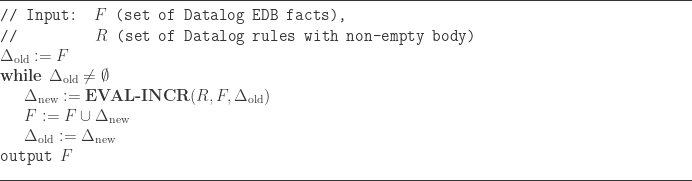
 as well as the subset of facts
  will consist of the set of rules
