Building A Graph Database Using Kafka

I previously showed how to build a relational database using Kafka. This time I’ll show how to build a graph database using Kafka. Just as with KarelDB, at the heart of our graph database will be the embedded key-value store, KCache.

Kafka as a Graph Database

The graph database that I’m most familiar with is HGraphDB, a graph database that uses HBase as its backend. More specifically, it uses the HBase client API, which allows it to integrate with not only HBase, but also any other data store that implements the HBase client API, such as Google BigTable. This leads to an idea. Rather than trying to build a new graph database around KCache entirely from scratch, we can try to wrap KCache with the HBase client API.

HBase is an example of a wide column store, also known as an extensible record store. Like its predecessor BigTable, it allows any number of column values to be associated with a key, without requiring a schema. For this reason, a wide column store can also be seen as two-dimensional key-value store.1

I’ve implemented KStore as a wide column store (or extensible record store) abstraction for Kafka that relies on KCache under the covers. KStore implements the HBase client API, so it can be used wherever the HBase client API is supported.

Let’s try to use KStore with HGraphDB. After installing and starting the Gremlin console, we install KStore and HGraphDB.

$ ./bin/gremlin.sh

         \,,,/
         (o o)
-----oOOo-(3)-oOOo-----
plugin activated: tinkerpop.server
plugin activated: tinkerpop.utilities
plugin activated: tinkerpop.tinkergraph

gremlin> :install org.apache.hbase hbase-client 2.2.1
gremlin> :install org.apache.hbase hbase-common 2.2.1
gremlin> :install org.apache.hadoop hadoop-common 3.1.2
gremlin> :install io.kstore kstore 0.1.0
gremlin> :install io.hgraphdb hgraphdb 3.0.0
gremlin> :plugin use io.hgraphdb
 

After we restart the Gremlin console, we configure HGraphDB with the KStore connection class and the Kafka bootstrap servers.2 We can then issue Gremlin commands against Kafka.

$ ./bin/gremlin.sh

         \,,,/
         (o o)
-----oOOo-(3)-oOOo-----
plugin activated: tinkerpop.server
plugin activated: tinkerpop.utilities
plugin activated: io.hgraphdb
plugin activated: tinkerpop.tinkergraph

gremlin> cfg = new HBaseGraphConfiguration()\
......1> .set("hbase.client.connection.impl", "io.kstore.KafkaStoreConnection")\
......2> .set("kafkacache.bootstrap.servers", "localhost:9092")
==>io.hgraphdb.HBaseGraphConfiguration@41b0ae4c

gremlin> graph = new HBaseGraph(cfg)
==>hbasegraph[hbasegraph]

gremlin> g = graph.traversal()
==>graphtraversalsource[hbasegraph[hbasegraph], standard]

gremlin> v1 = g.addV('person').property('name','marko').next()
==>v[0371a1db-8768-4910-94e3-7516fc65dab3]

gremlin> v2 = g.addV('person').property('name','stephen').next()
==>v[3bbc9ce3-24d3-41cf-bc4b-3d95dbac6589]

gremlin> g.V(v1).addE('knows').to(v2).property('weight',2).iterate()
  

It works! HBaseGraph is now using Kafka as its storage backend.

Kafka as a Document Database

Now that we have a wide column store abstraction for Kafka in the form of KStore, let’s see what else we can do with it. Another database that uses the HBase client API is HDocDB, a document database for HBase. To use KStore with HDocDB, first we need to set hbase.client.connection.impl in our hbase-site.xml as follows.

<configuration>
    <property>
        <name>hbase.client.connection.impl</name>
        <value>io.kstore.KafkaStoreConnection</value>
    </property>
    <property>
        <name>kafkacache.bootstrap.servers</name>
        <value>localhost:9092</value>
    </property>
</configuration>

Now we can issue MongoDB-like commands against Kafka, using HDocDB.3

$ jrunscript -cp <hbase-conf-dir>:target/hdocdb-1.0.1.jar:../kstore/target/kstore-0.1.0.jar -f target/classes/shell/hdocdb.js -f -

nashorn> db.mycoll.insert( { _id: "jdoe", first_name: "John", last_name: "Doe" } )

nashorn> var doc = db.mycoll.find( { last_name: "Doe" } )[0]

nashorn> print(doc)
{"_id":"jdoe","first_name":"John","last_name":"Doe"}

nashorn> db.mycoll.update( { last_name: "Doe" }, { $set: { first_name: "Jim" } } )

nashorn> var doc = db.mycoll.find( { last_name: "Doe" } )[0]

nashorn> print(doc)
{"_id":"jdoe","first_name":"Jim","last_name":"Doe"}
  

Pretty cool, right?

Kafka as a Wide Column Store

Of course, there is no requirement to wrap KStore with another layer in order to use it. KStore can be used directly as a wide column store abstraction on top of Kafka. I’ve integrated KStore with the HBase Shell so that one can work directly with KStore from the command line.

$ ./kstore-shell.sh localhost:9092

hbase(main):001:0> create 'test', 'cf'
Created table test
Took 0.2328 seconds
=> Hbase::Table - test

hbase(main):003:0* list
TABLE
test
1 row(s)
Took 0.0192 seconds
=> ["test"]

hbase(main):004:0> put 'test', 'row1', 'cf:a', 'value1'
Took 0.1284 seconds

hbase(main):005:0> put 'test', 'row2', 'cf:b', 'value2'
Took 0.0113 seconds

hbase(main):006:0> put 'test', 'row3', 'cf:c', 'value3'
Took 0.0096 seconds

hbase(main):007:0> scan 'test'
ROW                                COLUMN+CELL
 row1                              column=cf:a, timestamp=1578763986780, value=value1
 row2                              column=cf:b, timestamp=1578763992567, value=value2
 row3                              column=cf:c, timestamp=1578763996677, value=value3
3 row(s)
Took 0.0233 seconds

hbase(main):008:0> get 'test', 'row1'
COLUMN                             CELL
 cf:a                              timestamp=1578763986780, value=value1
1 row(s)
Took 0.0106 seconds

hbase(main):009:0>

There’s no limit to the type of fun one can have with KStore. 🙂

Back to Graphs

Getting back to graphs, another popular graph database is JanusGraph, which is interesting because it has a pluggable storage layer. Some of the storage backends that it supports through this layer are HBase, Cassandra, and BerkeleyDB.

Of course, KStore can be used in place of HBase when configuring JanusGraph. Again, it’s simply a matter of configuring the KStore connection class in the JanusGraph configuration.

storage.hbase.ext.hbase.client.connection.impl: io.kstore.KafkaStoreConnection
storage.hbase.ext.kafkacache.bootstrap.servers: localhost:9092

However, we can do better when integrating JanusGraph with Kafka. JanusGraph can be integrated with any storage backend that supports a wide column store abstraction. When integrating with key-value stores such as BerkeleyDB, JanusGraph provides its own adapter for mapping a key-value store to a wide column store. Thus we can simply provide KCache to JanusGraph as a key-value store, and it will perform the mapping to a wide column store abstraction for us automatically.

I’ve implemented a new storage plugin for JanusGraph called janusgraph-kafka that does exactly this. Let’s try it out. After following the instructions here, we can start the Gremlin console.

$ ./bin/gremlin.sh

         \,,,/
         (o o)
-----oOOo-(3)-oOOo-----
plugin activated: tinkerpop.server
plugin activated: tinkerpop.tinkergraph
plugin activated: tinkerpop.hadoop
plugin activated: tinkerpop.spark
plugin activated: tinkerpop.utilities
plugin activated: janusgraph.imports

gremlin>  graph = JanusGraphFactory.open('conf/janusgraph-kafka.properties')
==>standardjanusgraph[io.kcache.janusgraph.diskstorage.kafka.KafkaStoreManager:[127.0.0.1]]

gremlin> g = graph.traversal()
==>graphtraversalsource[standardjanusgraph[io.kcache.janusgraph.diskstorage.kafka.KafkaStoreManager:[127.0.0.1]], standard]

gremlin> v1 = g.addV('person').property('name','marko').next()
==>v[4320]

gremlin> v2 = g.addV('person').property('name','stephen').next()
==>v[4104]

gremlin> g.V(v1).addE('knows').to(v2).property('weight',2).iterate()
  

Works like a charm.

Summary

In this and the previous post, I’ve shown how Kafka can be used as

I guess I could have titled this post “Building a Graph Database, Document Database, and Wide Column Store Using Kafka”, although that’s a bit long. In any case, hopefully I’ve shown that Kafka is a lot more versatile than most people realize.


Building A Graph Database Using Kafka

Building A Relational Database Using Kafka

In a previous post, I showed how Kafka can be used as the persistent storage for an embedded key-value store, called KCache. Once you have a key-value store, it can be used as the basis for other models such as documents, graphs, and even SQL. For example, CockroachDB is a SQL layer built on top of the RocksDB key-value store and YugaByteDB is both a document and SQL layer built on top of RocksDB. Other databases such as FoundationDB claim to be multi-model, because they support several types of models at once, using the key-value store as a foundation.

In this post I will show how KCache can be extended to implement a fully-functional relational database, called KarelDB1. In addition, I will show how today a database architecture can be assembled from existing open-source components, much like how web frameworks like Dropwizard came into being by assembling components such as a web server (Jetty), RESTful API framework (Jersey), JSON serialization framework (Jackson), and an object-relational mapping layer (JDBI or Hibernate).

Hello, KarelDB

Before I drill into the components that comprise KarelDB, first let me show you how to quickly get it up and running. To get started, download a release, unpack it, and then modify config/kareldb.properties to point to an existing Kafka broker. Then run the following:

$ bin/kareldb-start config/kareldb.properties

While KarelDB is still running, at a separate terminal, enter the following command to start up sqlline, a command-line utility for accessing JDBC databases.

$ bin/sqlline
sqlline version 1.8.0

sqlline> !connect jdbc:avatica:remote:url=http://localhost:8765 admin admin

sqlline> create table books (id int, name varchar, author varchar);
No rows affected (0.114 seconds)

sqlline> insert into books values (1, 'The Trial', 'Franz Kafka');
1 row affected (0.576 seconds)

sqlline> select * from books;
+----+-----------+-------------+
| ID |   NAME    |   AUTHOR    |
+----+-----------+-------------+
| 1  | The Trial | Franz Kafka |
+----+-----------+-------------+
1 row selected (0.133 seconds)

KarelDB is now at your service.

Kafka for Persistence

At the heart of KarelDB is KCache, an embedded key-value store that is backed by Kafka.  Many components use Kafka as a simple key-value store, including Kafka Connect and Confluent Schema Registry.  KCache not only generalizes this functionality, but provides a simple Map based API for ease of use.  In addition, KCache can use different implementations for the embedded key-value store that is backed by Kafka.

In the case of KarelDB, by default KCache is configured as a RocksDB cache that is backed by Kafka. This allows KarelDB to support larger datasets and faster startup times. KCache can also be configured to use an in-memory cache instead of RocksDB if desired.

Avro for Serialization and Schema Evolution

Kafka has pretty much adopted Apache Avro as its de facto data format, and for good reason.  Not only does Avro provide a compact binary format, but it has excellent support for schema evolution.  Such support is why the Confluent Schema Registry has chosen Avro as the first format for which it provides schema management.

KarelDB uses Avro to both define relations (tables), and serialize the data for those relations.  By using Avro, KarelDB gets schema evolution for free when executing an ALTER TABLE command.

sqlline> !connect jdbc:avatica:remote:url=http://localhost:8765 admin admin 

sqlline> create table customers (id int, name varchar);
No rows affected (1.311 seconds)

sqlline> alter table customers add address varchar not null;
Error: Error -1 (00000) : 
Error while executing SQL "alter table customers add address varchar not null": 
org.apache.avro.SchemaValidationException: Unable to read schema:
{
  "type" : "record",
  "name" : "CUSTOMERS",
  "fields" : [ {
    "name" : "ID",
    "type" : "int",
    "sql.key.index" : 0
  }, {
    "name" : "NAME",
    "type" : [ "null", "string" ],
    "default" : null
  } ]
}
using schema:
{
  "type" : "record",
  "name" : "CUSTOMERS",
  "fields" : [ {
    "name" : "ID",
    "type" : "int",
    "sql.key.index" : 0
  }, {
    "name" : "NAME",
    "type" : [ "null", "string" ],
    "default" : null
  }, {
    "name" : "ADDRESS",
    "type" : "string"
  } ]
}

sqlline> alter table customers add address varchar null;
No rows affected (0.024 seconds)

As you can see above, when we first try to add a column with a NOT NULL constraint, Avro rejects the schema change, because adding a new field with a NOT NULL constraint would cause deserialization to fail for older records that don’t have that field. When we instead add the same column with a NULL constraint, the ALTER TABLE command succeeds.

By using Avro for deserialization, a field (without a NOT NULL constraint) that is added to a schema will be appropriately populated with a default, or null if the field is optional. This is all automatically handled by the underlying Avro framework.

Another important aspect of Avro is that it defines a standard sort order for data, as well as a comparison function that operates directly on the binary-encoded data, without first deserializing it. This allows KarelDB to efficiently handle key range queries, for example.

Calcite for SQL

Apache Calcite is a SQL framework that handles query parsing, optimization, and execution, but leaves out the data store. Calcite allows for relational expressions to be pushed down to the data store for more efficient processing. Otherwise, Calcite can process the query using a built-in enumerable calling convention, that allows the data store to be represented as a set of tuples that can be accessed through an iterator interface. An embedded key-value store is a perfect representation for such a set of tuples, so KarelDB will handle key lookups and key range filtering (using Avro’s sort order support) but otherwise defer query processing to Calcite’s enumerable convention. One nice aspect of the Calcite project is that it continues to develop optimizations for the enumerable convention, which will automatically benefit KarelDB moving forward.

Calcite supports ANSI-compliant SQL, including some newer functions such as JSON_VALUE and JSON_QUERY.

sqlline> create table authors (id int, json varchar);
No rows affected (0.132 seconds)

sqlline> insert into authors 
       > values (1, '{"name":"Franz Kafka", "book":"The Trial"}');
1 row affected (0.086 seconds)

sqlline> insert into authors 
       > values (2, '{"name":"Karel Capek", "book":"R.U.R."}');
1 row affected (0.036 seconds)

sqlline> select json_value(json, 'lax $.name') as author from authors;
+-------------+
|   AUTHOR    |
+-------------+
| Franz Kafka |
| Karel Capek |
+-------------+
2 rows selected (0.027 seconds)

Omid for Transactions and MVCC

Although Apache Omid was originally designed to work with HBase, it is a general framework for supporting transactions on a key-value store. In addition, Omid uses the underlying key-value store to persist metadata concerning transactions. This makes it especially easy to integrate Omid with an existing key-value store such as KCache.

Omid actually requires a few features from the key-value store, namely multi-versioned data and atomic compare-and-set capability. KarelDB layers these features atop KCache so that it can take advantage of Omid’s support for transaction management. Omid utilizes these features of the key-value store in order to provide snapshot isolation using multi-version concurrency control (MVCC). MVCC is a common technique used to implement snapshot isolation in other relational databases, such as Oracle and PostgreSQL.

Below we can see an example of how rolling back a transaction will restore the state of the database before the transaction began.

sqlline> !autocommit off

sqlline> select * from books;
+----+-----------+-------------+
| ID |   NAME    |   AUTHOR    |
+----+-----------+-------------+
| 1  | The Trial | Franz Kafka |
+----+-----------+-------------+
1 row selected (0.045 seconds)

sqlline> update books set name ='The Castle' where id = 1;
1 row affected (0.346 seconds)

sqlline> select * from books;
+----+------------+-------------+
| ID |    NAME    |   AUTHOR    |
+----+------------+-------------+
| 1  | The Castle | Franz Kafka |
+----+------------+-------------+
1 row selected (0.038 seconds)

sqlline> !rollback
Rollback complete (0.059 seconds)

sqlline> select * from books;
+----+-----------+-------------+
| ID |   NAME    |   AUTHOR    |
+----+-----------+-------------+
| 1  | The Trial | Franz Kafka |
+----+-----------+-------------+
1 row selected (0.032 seconds)

Transactions can of course span multiple rows and multiple tables.

Avatica for JDBC

KarelDB can actually be run in two modes, as an embedded database or as a server. In the case of a server, KarelDB uses Apache Avatica to provide RPC protocol support. Avatica provides both a server framework that wraps KarelDB, as well as a JDBC driver that can communicate with the server using Avatica RPC.

One advantage of using Kafka is that multiple servers can all “tail” the same set of topics. This allows multiple KarelDB servers to run as a cluster, with no single-point of failure. In this case, one of the servers will be elected as the leader while the others will be followers (or replicas). When a follower receives a JDBC request, it will use the Avatica JDBC driver to forward the JDBC request to the leader. If the leader fails, one of the followers will be elected as a new leader.

Database by Components

Today, open-source libraries have achieved what component-based software development was hoping to do many years ago. With open-source libraries, complex systems such as relational databases can be assembled by integrating a few well-designed components, each of which specializes in one thing that it does particularly well.

Above I’ve shown how KarelDB is an assemblage of several existing open-source components:

Currently, KarelDB is designed as a single-node database, which can be replicated, but it is not a distributed database. Also, KarelDB is a plain-old relational database, and does not handle stream processing. For a distributed, stream-relational database, please consider using KSQL instead, which is production-proven.

KarelDB is still in its early stages, but give it a try if you’re interesting in using Kafka to back your plain-old relational data.

Building A Relational Database Using Kafka

Machine Learning with Kafka Graphs

As data has become more prevalent from the rise of cloud computing, mobile devices, and big data systems, methods to analyze that data have become more and more advanced, with machine learning and artificial intelligence algorithms epitomizing the state-of-the-art. There are many ways to use machine learning to analyze data in Kafka. Below I will show how machine learning can be performed with Kafka Graphs, a graph analytics library that is layered on top of Kafka Streams.

Graph Modeling

As described in “Using Apache Kafka to Drive Cutting-Edge Machine Learning“, a machine learning lifecycle is comprised of modeling and prediction. That article goes on to describe how to integrate models from libraries like TensorFlow and H20, whether through RPC or by embedding the model in a Kafka application. With Kafka Graphs, the graph is the model. Therefore, when using Kafka Graphs for machine learning, there is no need to integrate with an external machine learning library for modeling.

Recommender Systems

As an example of machine learning with Kafka Graphs, I will show how Kafka Graphs can be used as a recommender system1. Recommender systems are commonly used by companies such as Amazon, Netflix, and Spotify to predict the rating or preference a user would give to an item. In fact, the Netflix Prize was a competition that Netflix started to determine if an external party could devise an algorithm that could provide a 10% improvement over Netflix’s own algorithm. The competition resulted in a wave of innovation in algorithms that use collaborative filtering2, which is a method of prediction based on the ratings or behavior of other users in the system.

Singular Value Decomposition

Singular value decomposition (SVD) is a type of matrix factorization popularized by Simon Funk for use in a recommender system during the Netflix competition. When using Funk SVD3, also called regularized SVD, the user-item rating matrix is viewed as the product of two lower-dimensional matrices, one with a row for each user, and another with a column for each item. For example, a 5×5 ratings matrix might be factored into a 5×2 user-feature matrix and a 2×5 item-feature matrix.

\begin{bmatrix}      r_{11} & r_{12} & r_{13} & r_{14} & r_{15} \\      r_{21} & r_{22} & r_{23} & r_{24} & r_{25} \\      r_{31} & r_{32} & r_{33} & r_{34} & r_{35} \\      r_{41} & r_{42} & r_{43} & r_{44} & r_{45} \\      r_{51} & r_{52} & r_{53} & r_{54} & r_{55}  \end{bmatrix}  =  \begin{bmatrix}      u_{11} & u_{12} \\      u_{21} & u_{22} \\      u_{31} & u_{32} \\      u_{41} & u_{42} \\      u_{51} & u_{52}  \end{bmatrix}  \begin{bmatrix}      v_{11} & v_{12} & v_{13} & v_{14} & v_{15} \\      v_{21} & v_{22} & v_{23} & v_{24} & v_{25} \\  \end{bmatrix}

Matrix factorization with SVD actually takes the form of

R = U \Sigma V^T

where \Sigma 
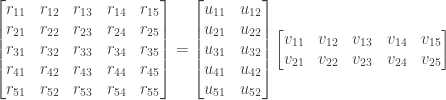
is a diagonal matrix of weights. The values in the row or column for the user-feature matrix or item-feature matrix are referred to as latent factors. The exact meanings of the latent factors are usually not discernible. For a movie, one latent factor might represent a specific genre, such as comedy or science-fiction; while for a user, one latent factor might represent gender while another might represent age group. The goal of Funk SVD is to extract these latent factors in order to predict the values of the user-item rating matrix.

While Funk SVD can only accommodate explicit interactions, in the form of numerical ratings, a team of researchers from AT&T enhanced Funk SVD to additionally account for implicit interactions, such as likes, purchases, and bookmarks. This enhanced algorithm is referred to as SVD++.4 During the Netflix competition, SVD++ was shown to generate more accurate predictions than Funk SVD.

Machine Learning on Pregel

Kafka Graphs provides an implementation of the Pregel programming model, so any algorithm written for the Pregel programming model can easily be supported by Kafka Graphs. For example, there are many machine learning algorithms written for Apache Giraph, an implementation of Pregel that runs on Apache Hadoop, so such algorithms are eligible to be run on Kafka Graphs as well, with only minor modifications. For Kafka Graphs, I’ve ported the SVD++ algorithm from Okapi, a library of machine learning and graph mining algorithms for Apache Giraph.

Running SVD++ on Kafka Graphs

In the rest of this post, I’ll show how you can run SVD++ using Kafka Graphs on a dataset of movie ratings. To set up your environment, install git, Maven, and Docker Compose. Then run the following steps:

git clone https://github.com/rayokota/kafka-graphs.git

cd kafka-graphs

mvn clean package -DskipTests

cd kafka-graphs-rest-app

docker-compose up
 

The last step above will launch Docker containers for a ZooKeeper instance, a Kafka instance, and two Kafka Graphs REST application instances. The application instances will each be assigned a subset of the graph vertices during the Pregel computation.

For our data, we will use the librec FilmTrust dataset, which is a relatively small set of 35497 movie ratings from users of the FilmTrust platform. The following command will import the movie ratings data into Kafka Graphs:

java \
  -cp target/kafka-graphs-rest-app-1.2.2-SNAPSHOT.jar \
  -Dloader.main=io.kgraph.tools.importer.GraphImporter \
  org.springframework.boot.loader.PropertiesLauncher 127.0.0.1:9092 \
  --edgesTopic initial-edges \
  --edgesFile ../kafka-graphs-core/src/test/resources/ratings.txt \
  --edgeParser io.kgraph.library.cf.EdgeCfLongIdFloatValueParser \
  --edgeValueSerializer org.apache.kafka.common.serialization.FloatSerializer
 

The remaining commands will all use the Kafka Graphs REST API. First we prepare the graph data for use by Pregel. The following command will group edges by the source vertex ID, and also ensure that topics for the vertices and edges have the same number of partitions.

curl -H "Content-type: application/json" -d '{ "algorithm":"svdpp",
  "initialEdgesTopic":"initial-edges", "verticesTopic":"vertices",
  "edgesGroupedBySourceTopic":"edges", "async":"false" }' \
  localhost:8888/prepare
 

Now we can configure the Pregel algorithm:

curl -H "Content-type: application/json" -d '{ "algorithm":"svdpp",
  "verticesTopic":"vertices", "edgesGroupedBySourceTopic":"edges", 
  "configs": { "random.seed": "0" } }' \
  localhost:8888/pregel
 

The above command will return a hexadecimal ID to represent the Pregel computation, such as a8d72fc8. This ID is used in the next command to start the Pregel computation.

curl -H "Content-type: application/json" -d '{  "numIterations": 6 }' \
  localhost:8888/pregel/{id}
 

You can now examine the state of the Pregel computation:

curl -H "Content-type: application/json" localhost:8888/pregel/{id}
 

Once the above command shows that the computation is no longer running, you can use the final state of the graph for predicting user ratings. For example, to predict the rating that user 2 would give to item 14, run the following command, using the same Pregel ID from previous steps:

java \
  -cp target/kafka-graphs-rest-app-1.2.2-SNAPSHOT.jar \
  -Dloader.main=io.kgraph.tools.library.SvdppPredictor \
  org.springframework.boot.loader.PropertiesLauncher localhost:8888 \
  {id} --user 2 --item 14
 

The above command will return the predicted rating, such as 2.3385806. You can predict other ratings by using the same command with different user and item IDs.

Summary

The Kafka ecosystem provides several ways to build a machine learning system. Besides the various machine learning libraries that can be directly integrated with a Kafka application, Kafka Graphs can be used to run any machine learning algorithm that has been adapted for the Pregel programming model. Since Kafka Graphs is a library built on top of Kafka Streams, we’ve essentially turned Kafka Streams into a distributed machine learning platform!

Machine Learning with Kafka Graphs

Fun with Confluent Schema Registry Extensions

The Confluent Schema Registry often serves as the heart of a streaming platform, as it provides centralized management and storage of the schemas for an organization. One feature of the Schema Registry that deserves more attention is its ability to incorporate pluggable resource extensions.

In this post I will show how resource extensions can be used to implement the following:

  1. Subject modes. For example, one might want to “freeze” a subject so that no further changes can be made.
  2. A Schema Registry browser. This is a complete single-page application for managing and visualizing schemas in a web browser.

Along the way I will show how to use the KCache library that I introduced in my last post.

Subject Modes

The first resource extension that I will demonstrate is one that provides support for subject modes. With this extension, a subject can be placed in “read-only” mode so that no further changes can be made to the subject. Also, an entire Schema Registry cluster can be placed in “read-only” mode. This may be useful, for example, when using Confluent Replicator to replicate Schema Registry from one Kafka cluster to another. If one wants to keep the two registries in sync, one could mark the Schema Registry that is the target of replication as “read-only”.

When implementing the extension, we want to associate a mode, either “read-only” or “read-write”, to a given subject (or * to indicate all subjects). The association needs to be persistent, so that it can survive a restart of the Schema Registry. We could use a database, but the Schema Registry already has a dependency on Kafka, so perhaps we can store the association in Kafka. This is a perfect use case for KCache, which is an in-memory cache backed by Kafka. Using an instance of KafkaCache, saving and retrieving the mode for a given subject is straightforward:

public class ModeRepository implements Closeable {

    // Used to represent all subjects
    public static final String SUBJECT_WILDCARD = "*";

    private final Cache<String, String> cache;

    public ModeRepository(SchemaRegistryConfig schemaRegistryConfig) {
        KafkaCacheConfig config =
            new KafkaCacheConfig(schemaRegistryConfig.originalProperties());
        cache = new KafkaCache<>(config, Serdes.String(), Serdes.String());
        cache.init();
    }

    public Mode getMode(String subject) {
        if (subject == null) subject = SUBJECT_WILDCARD;
        String mode = cache.get(subject);
        if (mode == null && subject.equals(SUBJECT_WILDCARD)) {
            // Default mode for top level
            return Mode.READWRITE;
        }
        return mode != null ? Enum.valueOf(Mode.class, mode) : null;
    }

    public void setMode(String subject, Mode mode) {
        if (subject == null) subject = SUBJECT_WILDCARD;
        cache.put(subject, mode.name());
    }

    @Override
    public void close() throws IOException {
        cache.close();
    }
}

Using the ModeRepository, we can provide a ModeResource class that provides REST APIs for saving and retrieving modes:

public class ModeResource {

    private static final int INVALID_MODE_ERROR_CODE = 42299;

    private final ModeRepository repository;
    private final KafkaSchemaRegistry schemaRegistry;

    public ModeResource(
        ModeRepository repository, 
        SchemaRegistry schemaRegistry
    ) {
        this.repository = repository;
        this.schemaRegistry = (KafkaSchemaRegistry) schemaRegistry;
    }

    @Path("/{subject}")
    @PUT
    public ModeUpdateRequest updateMode(
        @PathParam("subject") String subject,
        @Context HttpHeaders headers,
        @NotNull ModeUpdateRequest request
    ) {
        Mode mode;
        try {
            mode = Enum.valueOf(
                Mode.class, request.getMode().toUpperCase(Locale.ROOT));
        } catch (IllegalArgumentException e) {
            throw new RestConstraintViolationException(
                "Invalid mode. Valid values are READWRITE and READONLY.", 
                INVALID_MODE_ERROR_CODE);
        }
        try {
            if (schemaRegistry.isMaster()) {
                repository.setMode(subject, mode);
            } else {
                throw new RestSchemaRegistryException(
                    "Failed to update mode, not the master");
            }
        } catch (CacheException e) {
            throw Errors.storeException("Failed to update mode", e);
        }

        return request;
    }

    @Path("/{subject}")
    @GET
    public ModeGetResponse getMode(@PathParam("subject") String subject) {
        try {
            Mode mode = repository.getMode(subject);
            if (mode == null) {
                throw Errors.subjectNotFoundException();
            }
            return new ModeGetResponse(mode.name());
        } catch (CacheException e) {
            throw Errors.storeException("Failed to get mode", e);
        }
    }

    @PUT
    public ModeUpdateRequest updateTopLevelMode(
        @Context HttpHeaders headers,
        @NotNull ModeUpdateRequest request
    ) {
        return updateMode(ModeRepository.SUBJECT_WILDCARD, headers, request);
    }

    @GET
    public ModeGetResponse getTopLevelMode() {
        return getMode(ModeRepository.SUBJECT_WILDCARD);
    }
}

Now we need a filter to reject requests that attempt to modify a subject when it is in read-only mode:

@Priority(Priorities.AUTHORIZATION)
public class ModeFilter implements ContainerRequestFilter {

    private static final Set<ResourceActionKey> subjectWriteActions = 
        new HashSet<>();

    private ModeRepository repository;

    @Context
    ResourceInfo resourceInfo;

    @Context
    UriInfo uriInfo;

    @Context
    HttpServletRequest httpServletRequest;

    static {
        initializeSchemaRegistrySubjectWriteActions();
    }

    private static void initializeSchemaRegistrySubjectWriteActions() {
        subjectWriteActions.add(
            new ResourceActionKey(SubjectVersionsResource.class, "POST"));
        subjectWriteActions.add(
            new ResourceActionKey(SubjectVersionsResource.class, "DELETE"));
        subjectWriteActions.add(
            new ResourceActionKey(SubjectsResource.class, "DELETE"));
        subjectWriteActions.add(
            new ResourceActionKey(ConfigResource.class, "PUT"));
    }

    public ModeFilter(ModeRepository repository) {
        this.repository = repository;
    }

    @Override
    public void filter(ContainerRequestContext requestContext) {
        Class resource = resourceInfo.getResourceClass();
        String restMethod = requestContext.getMethod();
        String subject = uriInfo.getPathParameters().getFirst("subject");

        Mode mode = repository.getMode(subject);
        if (mode == null) {
            // Check the top level mode
            mode = repository.getMode(ModeRepository.SUBJECT_WILDCARD);
        }
        if (mode == Mode.READONLY) {
            ResourceActionKey key = new ResourceActionKey(resource, restMethod);
            if (subjectWriteActions.contains(key)) {
                requestContext.abortWith(
                    Response.status(Response.Status.UNAUTHORIZED)
                        .entity("Subject is read-only.")
                        .build());
            }
        }
    }

    private static class ResourceActionKey {

        private final Class resourceClass;
        private final String restMethod;

        public ResourceActionKey(Class resourceClass, String restMethod) {
            this.resourceClass = resourceClass;
            this.restMethod = restMethod;
        }

        ...
    }
}

Finally, the resource extension simply creates the mode repository and then registers the resource and the filter:

public class SchemaRegistryModeResourceExtension 
    implements SchemaRegistryResourceExtension {

    private ModeRepository repository;

    @Override
    public void register(
        Configurable<?> configurable,
        SchemaRegistryConfig schemaRegistryConfig,
        SchemaRegistry schemaRegistry
    ) {
        repository = new ModeRepository(schemaRegistryConfig);
        configurable.register(new ModeResource(repository, schemaRegistry));
        configurable.register(new ModeFilter(repository));
    }

    @Override
    public void close() throws IOException {
        repository.close();
    }
}

The complete source code listing can be found here.

To use our new resource extension, we first copy the extension jar (and the KCache jar) to ${CONFLUENT_HOME}/share/java/schema-registry. Next we add the following to ${CONFLUENT_HOME}/etc/schema-registry/schema-registry.properties:

kafkacache.bootstrap.servers=localhost:9092
resource.extension.class=io.yokota.schemaregistry.mode.SchemaRegistryModeResourceExtension

Now after we start the Schema Registry, we can save and retrieve modes for subjects via the REST API:

$ curl -X PUT -H "Content-Type: application/json" \
  http://localhost:8081/mode/topic-key --data '{"mode": "READONLY"}'
{"mode":"READONLY"}

$ curl localhost:8081/mode/topic-key
{"mode":"READONLY"}

$ curl -X POST -H "Content-Type: application/vnd.schemaregistry.v1+json" \
  --data '{ "schema": "{ \"type\": \"string\" }" }' \
  http://localhost:8081/subjects/topic-key/versions                                          
Subject is read-only.

It works!

A Schema Registry Browser

Resource extensions can not only be used to add new REST APIs to the Schema Registry; they can also be used to add entire web-based user interfaces. As a demonstration, I’ve developed a resource extension that provides a Schema Registry browser by bundling a single-page application based on Vue.js, which resides here. To use the Schema Registry browser, place the resource extension jar in ${CONFLUENT_HOME}/share/java/schema-registry and then add the following properties to ${CONFLUENT_HOME}/etc/schema-registry/schema-registry.properties:1

resource.static.locations=static
resource.extension.class=io.yokota.schemaregistry.browser.SchemaRegistryBrowserResourceExtension

The resource extension merely indicates which URLs should use the static resources:

public class SchemaRegistryBrowserResourceExtension 
    implements SchemaRegistryResourceExtension {

    @Override
    public void register(
        Configurable<?> configurable,
        SchemaRegistryConfig schemaRegistryConfig,
        SchemaRegistry kafkaSchemaRegistry
    ) throws SchemaRegistryException {
        configurable.property(ServletProperties.FILTER_STATIC_CONTENT_REGEX, 
            "/(static/.*|.*\\.html|.*\\.js)");
    }

    @Override
    public void close() {
    }
}

Once we start the Schema Registry and navigate to http://localhost:8081/index.html, we will be greeted with the home page of the Schema Registry browser:

From the Entities dropdown, we can navigate to a listing of all subjects:

If we view a specific subject, we can see the complete version history for the subject, with schemas nicely formatted:

I haven’t shown all the functionality of the Schema Registry browser, but it supports all the APIs that are available through REST, including creating schemas, retrieving schemas by ID, etc.

Hopefully this post has inspired you to create your own resource extensions for the Confluent Schema Registry. You might even have fun. 🙂

Fun with Confluent Schema Registry Extensions

KCache: An In-Memory Cache Backed by Kafka

Last year, Jay Kreps wrote a great article titled It’s Okay to Store Data in Apache Kafka, in which he discusses a variety of ways to use Kafka as a persistent store. In one of the patterns, Jay describes how Kafka can be used to back an in-memory cache:

You may have an in-memory cache in each instance of your application that is fed by updates from Kafka. A very simple way of building this is to make the Kafka topic log compacted, and have the app simply start fresh at offset zero whenever it restarts to populate its cache.

After reading the above, you may be thinking, “That’s what I want to do. How do I do it?”

I will now describe exactly how.

Roughly, there are two approaches.

In the first approach, you would

  1. Create a compacted topic in Kafka.
  2. Create a Kafka consumer that will never commit its offsets, and will start by reading from the beginning of the topic.
  3. Have the consumer initially read all records and insert them, in order, into an in-memory cache.
  4. Have the consumer continue to poll the topic in a background thread, updating the cache with new records.
  5. To insert a new record into the in-memory cache, use a Kafka producer to send the record to the topic, and wait for the consumer to read the new record and update the cache.
  6. To remove a record from the in-memory cache, use a Kafka producer to send a record with the given key and a null value (such a record is called a tombstone), and wait for the consumer to read the tombstone and remove the corresponding record from the cache.

In the second approach, you would instead use KCache, a small library that neatly wraps all of the above functionality behind a simple java.util.Map interface.

import io.kcache.*;

String bootstrapServers = "localhost:9092";
Cache<String, String> cache = new KafkaCache<>(
    bootstrapServers,
    Serdes.String(),  // for serializing/deserializing keys
    Serdes.String()   // for serializing/deserializing values
);
cache.init();  // creates topic, initializes cache, consumer, and producer
cache.put("Kafka", "Rocks");
String value = cache.get("Kafka");  // returns "Rocks"
cache.remove("Kafka");
cache.close();  // shuts down the cache, consumer, and producer

That’s it!

The choice is yours. 🙂

KCache: An In-Memory Cache Backed by Kafka

KDatalog: Kafka as a Datalog Engine

In previous posts, I had discussed how Kafka can be used for both stream-relational processing as well as graph processing. I will now show how Kafka can also be used to process Datalog programs.

The Datalog Language

Datalog 1 is a declarative logic programming language that is used as the query language for databases such as Datomic and LogicBlox.2 Both relational queries and graph-based queries can be expressed in Datalog, so in one sense it can be seen as a unifying or foundational database language. 3

Finite Model Theory

To mathematicians, both graphs and relations can be viewed as finite models. Finite model theory has been described as “the backbone of database theory”4. When SQL was developed, first-order logic was used as its foundation since it was seen as sufficient for expressing any database query that might ever be needed. Later theoreticians working in finite model theory were better able to understand the limits on the expressivity of first-order logic.

For example, Datalog was shown to be able to express queries involving transitive closure, which cannot be expressed in first-order logic nor in relational algebra, since relational algebra is equivalent to first-order logic.5 This led to the addition of the WITH RECURSIVE clause to SQL-99 in order to support transitive closure queries against relational databases.

Facts and Rules

Below is an example Datalog program.

  
parent(’Isabella’, ’Ella’).
parent(’Ella’, ’Ben’).
parent(’Daniel’, ’Ben’).
sibling(X, Y) :- parent(X, Z), parent(Y, Z), X̸ != Y.
  

The Datalog program above consists of 3 facts and 1 rule.6 A rule has a head and a body (separated by the :- symbol). The body is itself a conjunction of subgoals (separated by commas). The symbols X, Y, and Z are variables, while ‘Isabella’, ‘Ella’, ‘Ben’, and ‘Daniel’ are constants.

In the above program, the facts state that Isabella has a parent named Ella, Ella has a parent named Ben, and Daniel has a parent named Ben. The rule states that if there exist two people (X and Y) who are not the same (X != Y) and who have the same parent (Z), then they are siblings. Thus we can see that Ella and Daniel are siblings.

The initial facts of a Datalog program are often referred to as the extensional database (EDB), while the remaining rules define the intensional database (IDB). When evaluating a Datalog program, we use the extensional database as input to the rules in order to output the intensional database.

Datalog Evaluation

There are several ways to evaluate a Datalog program. One of the more straightforward algorithms is called semi-naive evaluation. In semi-naive evaluation, we use the most recently generated facts (\Delta_\text{old}) to satisfy one subgoal, and all facts F to satisfy the remaining subgoals, which generates a new set of facts (\Delta_\text{new}). These new facts are then used for the next evaluation round, and we continue iteratively until no new facts are derived.7 The algorithm is shown below, where \textbf{EVAL-INCR} is the method of satisfying subgoals just described.

\line(1,0){500} \\  \texttt{// Input: } F \texttt{ (set of Datalog EDB facts),} \\  \texttt{//}\hspace{56pt} R \texttt{ (set of Datalog rules with non-empty body)} \\  \Delta_\text{old} := F \\  \textbf{while } \Delta_\text{old} \neq \emptyset \\  \indent\Delta_\text{new} := \textbf{EVAL-INCR}(R,F,\Delta_\text{old}) \\  \indent F := F \cup \Delta_\text{new} \\  \indent\Delta_\text{old} := \Delta_\text{new} \\  \texttt{output } F \\  \line(1,0){500}

Semi-naive evaluation is essentially how incremental view maintenance is performed in relational databases.

So how might we use Kafka to evaluate Datalog programs? Well, it turns out that researchers have shown how to perform distributed semi-naive evaluation of Datalog programs on Pregel, Google’s framework for large-scale graph processing. Since Kafka Graphs supports Pregel, we can use Kafka Graphs to evaluate Datalog programs as well.

Datalog on Pregel

The general approach for implementing distributed semi-naive evaluation on Pregel is to treat each constant in the facts, such as ‘Ella’ and ‘Daniel’, as a vertex in a complete graph.8 The value of each vertex will be the complete set of rules R as well as the subset of facts F that reference the constant represented by the vertex. During each round of the semi-naive algorithm, a given vertex will resolve the subgoals with the facts that it has and then send facts or partial rules to other vertices if necessary. That means that each round will be comprised of one or more Pregel supersteps, since vertices receive messages that were sent in the previous superstep.

Beyond the straightforward approach described above9, many enhancements can be made, such as efficient grouping of vertices into super-vertices, rule rewriting, and support for recursive aggregates.10

Datalog Processing With Kafka Streams

Based on existing research, we can adapt the above approach to Kafka Graphs, which I call KDatalog.11

Assuming our Datalog program is in a file named siblings.txt, we first use KDatalog to parse the program and construct a graph consisting of vertices for the constants in the program, with edges between every pair of vertices. As mentioned, the initial value of the vertex for a given constant c will consist of the set of rules R as well as the subset of facts F that contain c.

    
    StreamsBuilder builder = new StreamsBuilder();
    Properties producerConfig = ...
    FileReader reader = new FileReader("siblings.txt");
    KGraph<String, String, String> graph = 
        KDatalog.createGraph(builder, producerConfig, reader);
    

We can then use this graph with KDatalog’s implementation of distributed semi-naive evaluation on Pregel, which is called DatalogComputation. After the computation terminates, the output of the algorithm will be the union of the values at every vertex.

Since KDatalog uses Kafka Graphs, and Kafka Graphs is built with Kafka Streams, we are essentially using Kafka Streams as a distributed Datalog engine.

The Future of Datalog

Datalog has recently enjoyed somewhat of a resurgence, as it has found successful application in a wide variety of areas, including data integration, information extraction, networking, program analysis, security, and cloud computing.12 Datalog has even been used to express conflict-free replicated data types (CRDTs) in distributed systems. If interest in Datalog continues to grow, perhaps Kafka will play an important role in helping enterprises use Datalog for their business needs.


KDatalog: Kafka as a Datalog Engine

Kafka Graphs: Graph Analytics with Apache Kafka

As the 2018 Apache Kafka Report has shown, Kafka has become mission-critical to enterprises of all sizes around the globe. Although there are many similar technologies in the field today, none have the equivalent of the thriving ecosystem that has developed around Kafka. Frameworks like Kafka Connect, Kafka Streams, and KSQL have enabled a much wider variety of scenarios to be addressed by Kafka. We are witnessing the growth of an entire technology market, distributed streaming, that resembles how the relational database market grew to take hold of enterprises at the end of the last century.

Kafka Graphs is a new framework that extends Kafka Streams to provide distributed graph analytics. It provides both a library for graph transformations as well as a distributed platform for executing graph algorithms. Kafka Graphs was inspired by other platforms for graph analytics, such as Apache Flink Gelly, Apache Spark GraphX, and Apache Giraph, but unlike these other frameworks it does not require anything other than what is already provided by the Kafka abstraction funnel.

Graph Representation and Transformations

A graph in Kafka Graphs is represented by two tables from Kafka Streams, one for vertices and one for edges. The vertex table is comprised of an ID and a vertex value, while the edge table is comprised of a source ID, target ID, and edge value.

KTable<Long, Long> vertices = ...
KTable<Edge<Long>, Long> edges = ...
KGraph<Long, Long, Long> graph = new KGraph<>(
    vertices, 
    edges, 
    GraphSerialized.with(Serdes.Long(), Serdes.Long(), Serdes.Long())
);

Once a graph is created, graph transformations can be performed on it. For example, the following will compute the sum of the values of all incoming neighbors for each vertex.

graph.reduceOnNeighbors(new SumValues(), EdgeDirection.IN);

Pregel-Based Graph Algorithms

Kafka Graphs provides a number of graph algorithms based on the vertex-centric approach of Pregel. The vertex-centric approach allows a computation to “think like a vertex” so that it only need consider how the value of a vertex should change based on messages sent from other vertices. The following algorithms are provided by Kafka Graphs:

  1. Breadth-first search (BFS): given a source vertex, determines the minimum number of hops to reach every other vertex.
  2. Label propagation (LP): finds communities in a graph by propagating labels between neighbors.
  3. Local clustering coefficient (LCC): computes the degree of clustering for each vertex as determined by the ratio between the number of triangles a vertex closes with its neighbors to the maximum number of triangles it could close.
  4. Multiple-source shortest paths (MSSP): given a set of source vertices, finds the shortest paths from these vertices to all other vertices.
  5. PageRank (PR): measures the rank or popularity of each vertex by propagating influence between vertices.
  6. Single-source shortest paths (SSSP): given a source vertex, finds the shortest paths to all other vertices.
  7. Weakly connected components (WCC): determines the weakly connected component for each vertex.

For example, here is the implementation of the single-source shortest paths (SSSP) algorithm:

public final class SSSPComputeFunction 
  implements ComputeFunction<Long, Double, Double, Double> {

  public void compute(
    int superstep,
    VertexWithValue<Long, Double> vertex,
    Map<Long, Double> messages,
    Iterable<EdgeWithValue<Long, Double>> edges,
    Callback<Long, Double, Double> cb) {

    double minDistance = vertex.id().equals(srcVertexId)
      ? 0d : Double.POSITIVE_INFINITY;

    for (Double message : messages.values()) {
      minDistance = Math.min(minDistance, message);
    }

    if (minDistance < vertex.value()) {
      cb.setNewVertexValue(minDistance);
      for (EdgeWithValue<Long, Double> edge : edges) {
        double distance = minDistance + edge.value();
        cb.sendMessageTo(edge.target(), distance);
      }
    }
  }
}

Custom Pregel-based graph algorithms can also be added by implementing the ComputeFunction interface.

Distributed Graph Processing

Since Kafka Graphs is built on top of Kafka Streams, it is able to leverage the underlying partitioning scheme of Kafka Streams in order to support distributed graph processing. To facilitate running graph algorithms in a distributed manner, Kafka Graphs provides a REST application for managing graph algorithm executions.

java -jar kafka-graphs-rest-app-0.1.0.jar \
  --kafka.graphs.bootstrapServers=localhost:9092 \
  --kafka.graphs.zookeeperConnect=localhost:2181

When multiple instantiations of the REST application are started on different hosts, all configured with the same Kafka and ZooKeeper servers, they will automatically coordinate with each other to partition the set of vertices when executing a graph algorithm. When a REST request is sent to one host, it will automatically proxy the request to the other hosts if necessary.

More information on the REST application can be found here.

Summary

Kafka Graphs is a new addition to the rapidly expanding ecosystem surrounding Apache Kafka. Kafka Graphs is still in its early stages, but please feel to try it and suggest improvements if you have a need to perform distributed graph analytics with Kafka.

Kafka Graphs: Graph Analytics with Apache Kafka

Embedding Kafka Connect in Kafka Streams + KSQL

Previously I presented the Kafka abstraction funnel and how it provides a simple yet powerful tool for writing applications that use Apache Kafka.  In this post I will show how these abstractions also provide a straightforward means of interfacing with Kafka Connect, so that applications that use Kafka Streams and KSQL can easily integrate with external systems like MySQL, Elasticsearch, and others.1

This is a somewhat lengthy post, so feel free to skip to the summary below.

Twins Separated at Birth?

Normally when using Kafka Connect, one would launch a cluster of Connect workers to run a combination of source connectors, that pull data from an external system into Kafka, and sink connectors, that push data from Kafka to an external system.  Once the data is in Kafka, one could then use Kafka Streams or KSQL to perform stream processing on the data.

Let’s take a look at two of the primary abstractions in Kafka Connect, the SourceTask and the SinkTask. The heart of the SourceTask class is the poll() method, which returns data from the external system.

/**
 * SourceTask is a Task that pulls records from another system for 
 * storage in Kafka.
 */
public abstract class SourceTask implements Task {
    ...

    public abstract void start(Map<String, String> props);

    public abstract List<SourceRecord> poll() 
        throws InterruptedException;

    public abstract void stop();

    ...
}

Likewise, the heart of the SinkTask is the put(Collection<SinkRecord> records) method, which sends data to the external system.

/**
 * SinkTask is a Task that takes records loaded from Kafka and 
 * sends them to another system.
 */
public abstract class SinkTask implements Task {
    ...

    public abstract void start(Map<String, String> props);

    public abstract void put(Collection<SinkRecord> records);

    public void flush(
        Map<TopicPartition, OffsetAndMetadata> currentOffsets) {
    }

    public abstract void stop();

    ...
}

Do those Kafka Connect classes remind of us anything in the Kafka abstraction funnel? Yes, indeed, the Consumer and Producer interfaces. Here is the Consumer:

/**
 * A client that consumes records from a Kafka cluster.
 */
public interface Consumer<K, V> extends Closeable {
    ...

    public void subscribe(
        Pattern pattern, ConsumerRebalanceListener callback);

    public ConsumerRecords<K, V> poll(long timeout);

    public void unsubscribe();

    public void close();

    ...
}

And here is the Producer:

/**
 * A Kafka client that publishes records to the Kafka cluster.
 */
public interface Producer<K, V> extends Closeable {
     ...

    Future<RecordMetadata> send(
        ProducerRecord<K, V> record, Callback callback);

    void flush();

    void close();

    ...
}

There are other methods in those interfaces that I’ve elided, but the above methods are the primary ones used by Kafka Streams.

Connect, Meet Streams

The Connect APIs and the Producer-Consumer APIs are very similar. Perhaps we can create implementations of the Producer-Consumer APIs that merely delegate to the Connect APIs. But how would we plug in our new implementations into Kafka Streams? Well, it turns out that Kafka Streams allows you to implement an interface that instructs it where to obtain a Producer and a Consumer:

/**
 * {@code KafkaClientSupplier} can be used to provide custom Kafka clients 
 * to a {@link KafkaStreams} instance.
 */
public interface KafkaClientSupplier {

    AdminClient getAdminClient(final Map<String, Object> config);

    Producer<byte[], byte[]> getProducer(Map<String, Object> config);

    Consumer<byte[], byte[]> getConsumer(Map<String, Object> config);

    ...
}

That’s just we want. Let’s try implementing a new Consumer that delegates to a Connect SourceTask. We’ll call it ConnectSourceConsumer.

public class ConnectSourceConsumer implements Consumer<byte[], byte[]> {

    private final SourceTask task;
    private final Converter keyConverter;
    private final Converter valueConverter;
    ...
    
    public ConsumerRecords<byte[], byte[]> poll(long timeout) {
        // Poll the Connect source task
        List<SourceRecord> records = task.poll();
        return records != null 
            ? new ConsumerRecords<>(convertRecords(records)) 
            : ConsumerRecords.empty();
    }

    // Convert the Connect records into Consumer records
    private ConsumerRecords<byte[], byte[]> convertRecords(
            List<SourceRecord> records) {

        for (final SourceRecord record : records) {
            byte[] key = keyConverter.fromConnectData(
                record.topic(), record.keySchema(), record.key());
            byte[] value = valueConverter.fromConnectData(
                record.topic(), record.valueSchema(), record.value());
            int partition = record.kafkaPartition() != null 
                ? record.kafkaPartition() : 0;
            final ConsumerRecord<byte[], byte[]> consumerRecord =
                    new ConsumerRecord<>(
                            record.topic(),
                            partition,
                            ...
                            key,
                            value);
            TopicPartition tp = new TopicPartition(
                record.topic(), partition);
            List<ConsumerRecord<byte[], byte[]>> consumerRecords = 
                result.computeIfAbsent(tp, k -> new ArrayList<>());
            consumerRecords.add(consumerRecord);
        }
        return new ConsumerRecords<>(result);
    }

    ...
}

And here is the new Producer that delegates to a Connect SinkTask, called ConnectSinkProducer.

public class ConnectSinkProducer implements Producer<byte[], byte[]> {

    private final SinkTask task;
    private final Converter keyConverter;
    private final Converter valueConverter;
    private final List<SinkRecord> recordBatch;
    ...

    public Future<RecordMetadata> send(
        ProducerRecord<byte[], byte[]> record, Callback callback) {
        convertRecords(Collections.singletonList(record));
        ...
    }

    // Convert the Connect records into Producer records
    private void convertRecords(
        List<ProducerRecord<byte[], byte[]>> records) {

        for (ProducerRecord<byte[], byte[]> record : records) {
            SchemaAndValue keyAndSchema = record.key() != null
                ? keyConverter.toConnectData(record.topic(), record.key())
                : SchemaAndValue.NULL;
            SchemaAndValue valueAndSchema = record.value() != null
                ? valueConverter.toConnectData(
                    record.topic(), record.value())
                : SchemaAndValue.NULL;
            int partition = record.partition() != null 
                ? record.partition() : 0;
            SinkRecord producerRecord = new SinkRecord(
                    record.topic(), partition,
                    keyAndSchema.schema(), keyAndSchema.value(),
                    valueAndSchema.schema(), valueAndSchema.value(),
                    ...);
            recordBatch.add(producerRecord);
        }
    }

    public void flush() {
        deliverRecords();
    }

    private void deliverRecords() {
        // Finally, deliver this batch to the sink
        try {
            task.put(new ArrayList<>(recordBatch));
            recordBatch.clear();
        } catch (RetriableException e) {
            // The batch will be reprocessed on the next loop.
        } catch (Throwable t) {
            throw new ConnectException("Unrecoverable exception:", t);
        }
    }

    ...
}

With our new classes in hand, let’s implement KafkaClientSupplier so we can let Kafka Streams know about them.

public class ConnectClientSupplier implements KafkaClientSupplier {
    ...
    
    public Producer<byte[], byte[]> getProducer(
        final Map<String, Object> config) {
        return new ConnectSinkProducer(config);
    }

    public Consumer<byte[], byte[]> getConsumer(
        final Map<String, Object> config) {
        return new ConnectSourceConsumer(config);
    }

    ...
}

Words Without Counts

We now have enough to run a simple function using Kafka Connect embedded in Kafka Streams.2. Let’s give it a whirl.

The following code performs the first half of a WordCount application, where the input is a stream of lines of text, and the output is a stream of words. However, instead of using Kafka for input/output, we use the JDBC Connector to read from a database table and write to another.

    Properties props = new Properties();
    props.put(StreamsConfig.APPLICATION_ID_CONFIG, "simple");
    props.put(StreamsConfig.CLIENT_ID_CONFIG, "simple-example-client");
    props.put(StreamsConfig.BOOTSTRAP_SERVERS_CONFIG, bootstrapServers);
    ...
    StreamsConfig streamsConfig = new StreamsConfig(props);

    Map<String, Object> config = new HashMap<>();
    ...
    ConnectStreamsConfig connectConfig = new ConnectStreamsConfig(config);

    // The JDBC source task configuration
    Map<String, Object> config = new HashMap<>();
    config.put(JdbcSourceConnectorConfig.CONNECTION_URL_CONFIG, jdbcUrl);
    config.put(JdbcSourceTaskConfig.TABLES_CONFIG, inputTopic);
    config.put(TaskConfig.TASK_CLASS_CONFIG, JdbcSourceTask.class.getName());
    TaskConfig sourceTaskConfig = new TaskConfig(config);

    // The JDBC sink task configuration
    Map<String, Object> config = new HashMap<>();
    config.put(JdbcSourceConnectorConfig.CONNECTION_URL_CONFIG, jdbcUrl);
    config.put(TaskConfig.TASK_CLASS_CONFIG, JdbcSinkTask.class.getName());
    TaskConfig sinkTaskConfig = new TaskConfig(config);

    StreamsBuilder builder = new StreamsBuilder();

    KStream<SchemaAndValue, SchemaAndValue> input = 
        builder.stream(inputTopic);

    KStream<SchemaAndValue, SchemaAndValue> output = input
        .flatMapValues(value -> {
            Struct lines = (Struct) value.value();
            String[] strs = lines.get("lines").toString()
                .toLowerCase().split("\\W+");
            List<SchemaAndValue> result = new ArrayList<>();
            for (String str : strs) {
                if (str.length() > 0) {
                    Schema schema = SchemaBuilder.struct().name("word")
                        .field("word", Schema.STRING_SCHEMA).build();
                    Struct struct = new Struct(schema).put("word", str);
                    result.add(new SchemaAndValue(schema, struct));
                }
            }
            return result;
        });

    output.to(outputTopic);

    streams = new KafkaStreams(builder.build(), streamsConfig,
            new ConnectClientSupplier("JDBC", connectConfig,
                    Collections.singletonMap(inputTopic, sourceTaskConfig),
                    Collections.singletonMap(outputTopic, sinkTaskConfig)));
    streams.start();
}

When we run the above example, it executes without involving Kafka at all!

This Is Not A Pipe3

Now that we have the first half of a WordCount application, let’s complete it. Normally we would just add a groupBy function to the above example, however that won’t work with our JDBC pipeline. The reason can be found in the JavaDoc for groupBy:

Because a new key is selected, an internal repartitioning topic will be created in Kafka. This topic will be named “${applicationId}-XXX-repartition”, where “applicationId” is user-specified in StreamsConfig via parameter APPLICATION_ID_CONFIG, “XXX” is an internally generated name, and “-repartition” is a fixed suffix.

So Kafka Streams will try to create a new topic, and it will do so by using the AdminClient obtained from KafkaClientSupplier. Therefore, we could, if we chose to, create an implementation of AdminClient that creates database tables instead of Kafka topics. However, if we remember to think of Kafka as Unix pipes, all we want to do is restructure our previous WordCount pipeline from this computation:

to the following computation, where the database interactions are no longer represented by pipes, but rather by stdin and stdout:

This allows Kafka Streams to use Kafka Connect without going through Kafka as an intermediary. In addition, there is no need for a cluster of Connect workers as the Kafka Streams layer is directly instantiating and managing the necessary Connect components. However, wherever there is a pipe (|) in the above pipeline, we still want Kafka to hold the intermediate results.

WordCount With Kafka Connect

So let’s continue to use an AdminClient that is backed by Kafka. However, if we want to use Kafka for intermediate results, we need to modify the APIs in ConnectClientSupplier. We will now need this class to return instances of Producer and Consumer that delegate to Kafka Connect for the stream input and output, but to Kafka for intermediate results that are produced within the stream.

public class ConnectClientSupplier implements KafkaClientSupplier {

    private DefaultKafkaClientSupplier defaultSupplier = 
        new DefaultKafkaClientSupplier();
    private String connectorName;
    private ConnectStreamsConfig connectStreamsConfig;
    private Map<String, TaskConfig> sourceTaskConfigs;
    private Map<String, TaskConfig> sinkTaskConfigs;

    public ConnectClientSupplier(
        String connectorName, ConnectStreamsConfig connectStreamsConfig,
        Map<String, TaskConfig> sourceTaskConfigs,
        Map<String, TaskConfig> sinkTaskConfigs) {

        this.connectorName = connectorName;
        this.connectStreamsConfig = connectStreamsConfig;
        this.sourceTaskConfigs = sourceTaskConfigs;
        this.sinkTaskConfigs = sinkTaskConfigs;
    }

    ...

    @Override
    public Producer<byte[], byte[]> getProducer(
        Map<String, Object> config) {

        ProducerConfig producerConfig = new ProducerConfig(
            ProducerConfig.addSerializerToConfig(config, 
                new ByteArraySerializer(), new ByteArraySerializer()));
        Map<String, ConnectSinkProducer> connectProducers =
            sinkTaskConfigs.entrySet().stream()
                .collect(Collectors.toMap(Map.Entry::getKey,
                    e -> ConnectSinkProducer.create(
                        connectorName, connectStreamsConfig, 
                        e.getValue(), producerConfig)));

        // Return a Producer that delegates to Connect or Kafka
        return new WrappedProducer(
            connectProducers, defaultSupplier.getProducer(config));
    }

    @Override
    public Consumer<byte[], byte[]> getConsumer(
        Map<String, Object> config) {

        ConsumerConfig consumerConfig = new ConsumerConfig(
            ConsumerConfig.addDeserializerToConfig(config, 
                new ByteArrayDeserializer(), new ByteArrayDeserializer()));
        Map<String, ConnectSourceConsumer> connectConsumers =
            sourceTaskConfigs.entrySet().stream()
                .collect(Collectors.toMap(Map.Entry::getKey,
                    e -> ConnectSourceConsumer.create(
                        connectorName, connectStreamsConfig, 
                        e.getValue(), consumerConfig)));

        // Return a Consumer that delegates to Connect and Kafka
        return new WrappedConsumer(
            connectConsumers, defaultSupplier.getConsumer(config));
    }
    
    ...
}

The WrappedProducer simply sends a record to either Kafka or the appropriate Connect SinkTask, depending on the topic or table name.

public class WrappedProducer implements Producer<byte[], byte[]> {
    private final Map<String, ConnectSinkProducer> connectProducers;
    private final Producer<byte[], byte[]> kafkaProducer;

    @Override
    public Future<RecordMetadata> send(
        ProducerRecord<byte[], byte[]> record, Callback callback) {
        String topic = record.topic();
        ConnectSinkProducer connectProducer = connectProducers.get(topic);
        if (connectProducer != null) {
            // Send to Connect
            return connectProducer.send(record, callback);
        } else {
            // Send to Kafka
            return kafkaProducer.send(record, callback);
        }
    }

    ...
}

The WrappedConsumer simply polls Kafka and all the Connect SourceTask instances and then combines their results.

public class WrappedConsumer implements Consumer<byte[], byte[]> {
    private final Map<String, ConnectSourceConsumer> connectConsumers;
    private final Consumer<byte[], byte[]> kafkaConsumer;

    @Override
    public ConsumerRecords<byte[], byte[]> poll(long timeout) {
        Map<TopicPartition, List<ConsumerRecord<byte[], byte[]>>> records 
            = new HashMap<>();
        // Poll from Kafka
        poll(kafkaConsumer, timeout, records);
        for (ConnectSourceConsumer consumer : connectConsumers.values()) {
            // Poll from Connect
            poll(consumer, timeout, records);
        }
        return new ConsumerRecords<>(records);
    }

    private void poll(
        Consumer<byte[], byte[]> consumer, long timeout,
        Map<TopicPartition, List<ConsumerRecord<byte[], byte[]>>> records) {
        try {
            ConsumerRecords<byte[], byte[]> rec = consumer.poll(timeout);
            for (TopicPartition tp : rec.partitions()) {
                records.put(tp, rec.records(tp);
            }
        } catch (Exception e) {
            log.error("Could not poll consumer", e);
        }
    }
    
    ...
}

Finally we can use groupBy to implement WordCount.

    Properties props = new Properties();
    props.put(StreamsConfig.APPLICATION_ID_CONFIG, "simple");
    props.put(StreamsConfig.CLIENT_ID_CONFIG, "simple-example-client");
    props.put(StreamsConfig.BOOTSTRAP_SERVERS_CONFIG, bootstrapServers);
    ...
    StreamsConfig streamsConfig = new StreamsConfig(props);

    Map<String, Object> config = new HashMap<>();
    ...
    ConnectStreamsConfig connectConfig = new ConnectStreamsConfig(config);

    // The JDBC source task configuration
    Map<String, Object> config = new HashMap<>();
    config.put(JdbcSourceConnectorConfig.CONNECTION_URL_CONFIG, jdbcUrl);
    config.put(JdbcSourceTaskConfig.TABLES_CONFIG, inputTopic);
    config.put(TaskConfig.TASK_CLASS_CONFIG, JdbcSourceTask.class.getName());
    TaskConfig sourceTaskConfig = new TaskConfig(config);

    // The JDBC sink task configuration
    Map<String, Object> config = new HashMap<>();
    config.put(JdbcSourceConnectorConfig.CONNECTION_URL_CONFIG, jdbcUrl);
    config.put(TaskConfig.TASK_CLASS_CONFIG, JdbcSinkTask.class.getName());
    TaskConfig sinkTaskConfig = new TaskConfig(config);

    StreamsBuilder builder = new StreamsBuilder();

    KStream<SchemaAndValue, SchemaAndValue> input = builder.stream(inputTopic);

    KStream<SchemaAndValue, String> words = input
        .flatMapValues(value -> {
            Struct lines = (Struct) value.value();
            String[] strs = lines.get("lines").toString()
                .toLowerCase().split("\\W+");
            List<String> result = new ArrayList<>();
            for (String str : strs) {
                if (str.length() > 0) {
                    result.add(str);
                }
            }
            return result;
        });

    KTable<String, Long> wordCounts = words
        .groupBy((key, word) -> word, 
            Serialized.with(Serdes.String(), Serdes.String()))
        .count();

    wordCounts.toStream().map(
        (key, value) -> {
            Schema schema = SchemaBuilder.struct().name("word")
                    .field("word", Schema.STRING_SCHEMA)
                    .field("count", Schema.INT64_SCHEMA).build();
            Struct struct = new Struct(schema)
                .put("word", key).put("count", value);
            return new KeyValue<>(SchemaAndValue.NULL, 
                new SchemaAndValue(schema, struct));
        }).to(outputTopic);

    streams = new KafkaStreams(builder.build(), streamsConfig,
            new ConnectClientSupplier("JDBC", connectConfig,
                    Collections.singletonMap(inputTopic, sourceTaskConfig),
                    Collections.singletonMap(outputTopic, sinkTaskConfig)));
    streams.start();

When we run this WordCount application, it will use the JDBC Connector for input and output, and Kafka for intermediate results, as expected.

Connect, Meet KSQL

Since KSQL is built on top of Kafka Streams, with the above classes we get integration between Kafka Connect and KSQL for free, thanks to the Kafka abstraction funnel.

For example, here is a KSQL program to retrieve word counts that are greater than 100.

    Map<String, Object> config = new HashMap<>();
    ...
    ConnectStreamsConfig connectConfig = new ConnectStreamsConfig(config);

    // The JDBC source task configuration
    Map<String, Object> config = new HashMap<>();
    config.put(JdbcSourceConnectorConfig.CONNECTION_URL_CONFIG, jdbcUrl);
    config.put(JdbcSourceTaskConfig.TABLES_CONFIG, inputTopic);
    config.put(TaskConfig.TASK_CLASS_CONFIG, JdbcSourceTask.class.getName());
    TaskConfig sourceTaskConfig = new TaskConfig(config);

    KafkaClientSupplier clientSupplier = 
        new ConnectClientSupplier("JDBC", connectConfig,
                Collections.singletonMap(inputTopic, sourceTaskConfig),
                Collections.emptyMap());

    ksqlContext = KsqlContext.create(
        ksqlConfig, schemaRegistryClient, clientSupplier);

    ksqlContext.sql("CREATE STREAM WORD_COUNTS" 
        + " (ID int, WORD varchar, WORD_COUNT bigint)"
        + " WITH (kafka_topic='word_counts', value_format='AVRO', key='ID');";

    ksqlContext.sql("CREATE STREAM TOP_WORD_COUNTS AS "
        + " SELECT * FROM WORD_COUNTS WHERE WORD_COUNT > 100;";

When we run this example, it uses the JDBC Connector to read its input from a relational database. This is because we pass an instance of ConnectClientSupplier to the KsqlContext factory, in order to instruct the Kafka Streams layer underlying KSQL where to obtain the Producer and Consumer.4

Summary

With the above examples I’ve been able to demonstrate both

  1. the power of clean abstractions, especially as utilized in the Kafka abstraction funnel, and
  2. a promising method of integrating Kafka Connect with Kafka Streams and KSQL based on these abstractions.

Ironically, I have also shown that the Kafka abstraction funnel does not need to be tied to Kafka at all. It can be used with any system that provides implementations of the Producer-Consumer APIs, which reside at the bottom of the funnel. In this post I have shown how to plug in Kafka Connect at this level to achieve embedded Kafka Connect functionality within Kafka Streams. However, frameworks other than Kafka Connect could be used as well. In this light, Kafka Streams (as well as KSQL) can be viewed as a general stream processing platform in the same manner as Flink and Spark.

I hope you have enjoyed these excursions into some of the inner workings of Kafka Connect, Kafka Streams, and KSQL.

Embedding Kafka Connect in Kafka Streams + KSQL

The Hitchhiker’s Guide to Stream Processing

In my previous post I discussed some of the features of different stream processing platforms, but I did not touch on how one goes about choosing one.  In the book Kafka: The Definitive Guide, the authors provide some valuable advice on how to make a choice.  Below I present three additional tips for choosing a stream processing platform.

  1. Favor reuse over polyglot streaming.
  2. Try the Kafka abstraction funnel.
  3. Check out the Stream Processing Kickstarter project.

Favor Reuse Over Polyglot Streaming

One of the characteristics of many microservice architectures is the use of several different data stores, which is often referred to as polyglot persistence.  The idea is that each microservice should be responsible for its own data, which often leads to each microservice possibly introducing a different data store into the organization.   However, at my last company, Yammer, this led to an operational nightmare as we attempted to manage and develop expertise in a variety of data stores.  In the end, we decided to consolidate on one relational database (PostgreSQL) and one non-relational database (HBase).

The real underlying goal for data use in microservices is to eliminate coupling between business subdomains in an application, which can be better achieved by schema independence, rather than polyglot persistence.  Schema independence can easily be achieved by partitioning data properly within a single data store, using namespaces, schemas, or other techniques, and does not necessitate the use of polyglot persistence.

In a streaming architecture, one of the goals is to share data rather than to keep it siloed.  This is often referred to as turning the database inside-out, as achieved by many event-driven systems. This means that schemas need to be shared as well, which leads to the use of schema registries.  Consequently, it makes even less sense to use more than one streaming platform in an organization, which would lead to polyglot streaming.   Therefore, if your organization is already using a stream processing platform, perhaps in a different group from the one that you are in, try using that.

Try the Kafka Abstraction Funnel

Kafka has emerged as the foundation for stream processing in today’s enterprises.  Kafka provides a low-level Producer-Consumer API, but it also comes bundled with a stream processing framework called Kafka Streams, which has both a Processor API and a Streams DSL (that is built on top of the Processor API).  Additionally, Confluent (the company I work for) has just released KSQL, which is built on top of Kafka Streams.

These four layers (KSQL, the Kafka Streams DSL, the Kafka Streams Processor API, and the Producer-Consumer API) form a hierarchy of abstractions, which I refer to as the Kafka abstraction funnel.   In accordance with the 80-20 rule, the top of the funnel, KSQL, should be able to handle 80% of your use cases, and for the remaining 20%, you can drop down into the Kafka Streams DSL.  Likewise, the Kafka Streams DSL should be able to handle 80% of the use cases that KSQL cannot handle, and for the remaining 20%, you can drop down into the Kafka Streams Processor API.  Finally, at the bottom of the funnel is the Producer-Consumer API, which should be able to handle everything else.

The Kafka abstraction funnel is very easy to get started with, provides support for stream-relational processing, and simply builds on technologies already provided with Kafka.  Give it a try if you can.

I’ll have more to say about the power of the Kafka abstraction funnel in my next post.

Check Out the Stream Processing Kickstarter Project

Martin Kleppman has likened Kafka to Unix pipes, with the stream processor being the Unix program that reads from one pipe and writes to another.  However, if you’re using Kafka but you’ve not settled on the Kafka abstraction funnel, figuring out exactly which stream processor to use can be a bewildering task.

There are other posts that compare the different streaming platforms.  Often these comparisons show how to write a WordCount application, which has become the “Hello World” example of data processing.   However, most of the WordCount examples don’t actually show how to integrate with Kafka.  Therefore I’ve put together the Stream Processing Kickstarter that has the WordCount application written in each of the most popular streaming frameworks.  Furthermore, in each WordCount application, I show how to read textual data from a Kafka topic and then output the word counts to another Kafka topic.  Also, each example in the project can be easily executed against an embedded Kafka cluster by simply running a unit test.

Below I show the code for each WordCount application so you can get a sense what it is like to use each streaming platform.1

Beam

In Apache Beam, integration with Kafka is achieved by using a Kafka reader transform and a Kafka writer transform.

public class BeamWordCount implements WordCount {

  @Override
  public void countWords(
      String bootstrapServers, String zookeeperConnect,
      String inputTopic, String outputTopic) {

    PipelineOptions options = PipelineOptionsFactory.create();
    Pipeline p = Pipeline.create(options);

    KafkaIO.Read<String, String> reader = KafkaIO.<String, String>read()
        .withBootstrapServers(bootstrapServers)
        .withTopic(inputTopic)
        .withKeyDeserializer(StringDeserializer.class)
        .withValueDeserializer(StringDeserializer.class)
        .updateConsumerProperties(
            ImmutableMap.of(
                ConsumerConfig.AUTO_OFFSET_RESET_CONFIG, "earliest"));

    PCollection<String> input = p.apply(reader.withoutMetadata())
        .apply(MapElements
            .into(TypeDescriptors.strings())
            .via(KV::getValue))
        .apply(ParDo.of(new AddTimestampFn()));

    PCollection<String> windowedWords = input.apply(
        Window.<String>into(FixedWindows.of(Duration.standardSeconds(1)))
            .triggering(Repeatedly.forever(AfterPane.elementCountAtLeast(1)))
            .withAllowedLateness(Duration.ZERO)
            .accumulatingFiredPanes());

    PCollection<KV<String, Long>> wordCounts =
        windowedWords.apply(new CountWords());

    wordCounts.apply(KafkaIO.<String, Long>write()
        .withBootstrapServers(bootstrapServers)
        .withTopic(outputTopic)
        .withKeySerializer(StringSerializer.class)
        .withValueSerializer(LongSerializer.class));

    p.run().waitUntilFinish(Duration.standardSeconds(5));
  }

  @Override
  public void close() {
  }

  static class AddTimestampFn extends DoFn<String, String> {

    @ProcessElement
    public void processElement(ProcessContext c) {
      c.outputWithTimestamp(c.element(), Instant.now());
    }
  }

  static class ExtractWordsFn extends DoFn<String, String> {

    @ProcessElement
    public void processElement(ProcessContext c) {
      // Split the line into words.
      String[] words = c.element().toLowerCase().split("\\W+");

      // Output each word encountered into the output PCollection.
      for (String word : words) {
        if (!word.isEmpty()) {
          c.output(word);
        }
      }
    }
  }

  static class CountWords extends PTransform<PCollection<String>,
      PCollection<KV<String, Long>>> {
    @Override
    public PCollection<KV<String, Long>> expand(PCollection<String> lines) {

      // Convert lines of text into individual words.
      PCollection<String> words = lines.apply(
          ParDo.of(new ExtractWordsFn()));

      // Count the number of times each word occurs.
      PCollection<KV<String, Long>> wordCounts =
          words.apply(Count.perElement());

      return wordCounts;
    }
  }
}

Flink

The Flink example uses a Kafka source and a Kafka sink.

public class FlinkWordCount implements WordCount {

  @Override
  public void countWords(
      String bootstrapServers, String zookeeperConnect,
      String inputTopic, String outputTopic) throws Exception {

    Properties props = new Properties();
    props.put("bootstrap.servers", bootstrapServers);
    props.put("group.id", "testgroup");
    props.put("auto.offset.reset", "earliest");

    // set up the execution environment
    final StreamExecutionEnvironment env =
        StreamExecutionEnvironment.getExecutionEnvironment();

    DataStream<String> input = env
        .addSource(new FlinkKafkaConsumer011<>(
            inputTopic,
            new SimpleStringSchema(),
            props
        ));

    DataStream<Tuple2<String, Long>> counts = input
        .map(line -> line.toLowerCase().split("\\W+"))
        .flatMap((String[] tokens, Collector<Tuple2<String, Long>> out) -> {
          // emit the pairs with non-zero-length words
          Arrays.stream(tokens)
              .filter(t -> t.length() > 0)
              .forEach(t -> out.collect(new Tuple2<>(t, 1L)));
        })
        .keyBy(0)
        .sum(1);

    counts.addSink(
        new FlinkKafkaProducer011<>(
            outputTopic,
            new WordCountSerializer(outputTopic),
            props
        ));

    // execute program
    env.execute("Streaming WordCount Example");
  }

  @Override
  public void close() {
  }

  static class WordCountSerializer implements
      KeyedSerializationSchema<Tuple2<String, Long>>,
      java.io.Serializable {

    private final String outputTopic;

    public WordCountSerializer(String outputTopic) {
      this.outputTopic = outputTopic;
    }

    public byte[] serializeKey(Tuple2<String, Long> element) {
      return new StringSerializer().serialize(null, element.getField(0));
    }

    public byte[] serializeValue(Tuple2<String, Long> element) {
      return new LongSerializer().serialize(null, element.getField(1));
    }

    public String getTargetTopic(Tuple2<String, Long> element) {
      return outputTopic;
    }
  }
}

Kafka Streams

Kafka Streams, being built directly atop Kafka, has the simplest integration with Kafka.  An input stream is constructed directly from a Kafka topic and then later the data in the stream is sent directly to another Kafka topic.

public class KafkaStreamsWordCount implements WordCount {

  private KafkaStreams streams;

  @Override
  public void countWords(
      String bootstrapServers, String zookeeperConnect,
      String inputTopic, String outputTopic) {

    Properties props = new Properties();
    props.put(StreamsConfig.APPLICATION_ID_CONFIG, "wordcount");
    props.put(StreamsConfig.CLIENT_ID_CONFIG, "wordcount-example-client");
    props.put(StreamsConfig.BOOTSTRAP_SERVERS_CONFIG, bootstrapServers);
    props.put(
        StreamsConfig.DEFAULT_KEY_SERDE_CLASS_CONFIG,
        Serdes.String().getClass().getName()
    );
    props.put(
        StreamsConfig.DEFAULT_VALUE_SERDE_CLASS_CONFIG,
        Serdes.String().getClass().getName()
    );
    props.put(StreamsConfig.CACHE_MAX_BYTES_BUFFERING_CONFIG, 0);
    props.put(
        StreamsConfig.STATE_DIR_CONFIG,
        Utils.tempDirectory().getAbsolutePath()
    );

    StreamsBuilder builder = new StreamsBuilder();

    KStream<String, String> input = builder.stream(inputTopic);

    KTable<String, Long> wordCounts = input
        .flatMapValues(
            value -> Arrays.asList(value.toLowerCase().split("\\W+")))
        .groupBy((key, word) -> word)
        .count();

    wordCounts.toStream().to(
        outputTopic, Produced.with(Serdes.String(), Serdes.Long()));

    streams = new KafkaStreams(builder.build(), props);
    streams.start();
  }

  @Override
  public void close() {
    streams.close();
  }
}

Samza

Samza can also create streams directly from Kafka topics by using a Kafka system factory.

public class SamzaWordCount implements WordCount {

  @Override
  public void countWords(
      String bootstrapServers, String zookeeperConnect,
      String inputTopic, String outputTopic) {

    Map<String, String> configs = new HashMap<>();

    configs.put(JobConfig.JOB_NAME(), "word-count");
    configs.put(JobConfig.PROCESSOR_ID(), "1");
    configs.put(
        JobCoordinatorConfig.JOB_COORDINATION_UTILS_FACTORY,
        PassthroughCoordinationUtilsFactory.class.getName()
    );
    configs.put(
        JobCoordinatorConfig.JOB_COORDINATOR_FACTORY,
        PassthroughJobCoordinatorFactory.class.getName()
    );
    configs.put(
        TaskConfig.GROUPER_FACTORY(),
        SingleContainerGrouperFactory.class.getName()
    );
    configs.put(
        "systems.kafka.samza.factory",
        "org.apache.samza.system.kafka.KafkaSystemFactory"
    );
    configs.put("systems.kafka.producer.bootstrap.servers", bootstrapServers);
    configs.put("systems.kafka.consumer.zookeeper.connect", zookeeperConnect);
    configs.put("systems.kafka.samza.offset.default", "oldest");
    configs.put("systems.kafka.default.stream.replication.factor", "1");
    configs.put("job.default.system", "kafka");

    LocalApplicationRunner runner =
        new LocalApplicationRunner(new MapConfig(configs));
    runner.run(new WordCountApplication(inputTopic, outputTopic));
    runner.waitForFinish();
  }

  @Override
  public void close() {
  }

  static class WordCountApplication implements StreamApplication {

    private String inputTopic;
    private String outputTopic;

    public WordCountApplication(String inputTopic, String outputTopic) {
      this.inputTopic = inputTopic;
      this.outputTopic = outputTopic;
    }

    @Override
    public void init(StreamGraph graph, Config config) {
      MessageStream<KV<String, String>> words =
          graph.getInputStream(
              inputTopic, KVSerde.of(new StringSerde(), new StringSerde()));
      OutputStream<KV<String, Long>> counts =
          graph.getOutputStream(
              outputTopic, KVSerde.of(new StringSerde(), new LongSerde()));

      words.flatMap(kv -> Arrays.asList(kv.value.toLowerCase().split("\\W+")))
          .window(Windows.keyedTumblingWindow(
              (String kv) -> kv, Duration.ofSeconds(1),
              () -> 0L, (m, prevCount) -> prevCount + 1,
              new StringSerde(), new LongSerde()
          )
              .setEarlyTrigger(Triggers.repeat(Triggers.count(1)))
              .setAccumulationMode(AccumulationMode.ACCUMULATING), "count")
          .map(windowPane -> {
            String word = windowPane.getKey().getKey();
            long count = windowPane.getMessage();
            return KV.of(word, count);
          })
          .sendTo(counts);
    }
  }
}

Spark

Spark structured streaming can create streams for Kafka by specifying a Kafka format.  Spark only supports writing strings or byte arrays to Kafka, so we use a Spark UDF to convert the count from a Long to a byte[].

public class SparkWordCount implements WordCount, java.io.Serializable {

  private StreamingQuery query;

  @Override
  public void countWords(
      String bootstrapServers, String zookeeperConnect,
      String inputTopic, String outputTopic) {

    SparkSession spark = SparkSession
        .builder()
        .appName("JavaStructuredKafkaWordCount")
        .config("spark.master", "local[*]")
        .getOrCreate();

    spark.udf().register(
        "serializeLong", new SparkLongSerializer(), DataTypes.BinaryType);

    // Create DataSet representing the stream of input lines from kafka
    Dataset<String> lines = spark
        .readStream()
        .format("kafka")
        .option("kafka.bootstrap.servers", bootstrapServers)
        .option("subscribe", inputTopic)
        .option("startingOffsets", "earliest")
        .load()
        .selectExpr("CAST(value as STRING)")
        .as(Encoders.STRING());

    // Generate running word count
    Dataset<Row> wordCounts = lines.flatMap(
        (FlatMapFunction<String, String>) x ->
            Arrays.asList(x.toLowerCase().split("\\W+"))
                .iterator(),
        Encoders.STRING()
    ).groupBy("value").count();

    // Start running the query that outputs the running counts to Kafka
    query = wordCounts
        .selectExpr("CAST(value AS STRING) key",
            "CAST(serializeLong(count) AS BINARY) value")
        .writeStream()
        .outputMode("update")
        .format("kafka")
        .option("kafka.bootstrap.servers", bootstrapServers)
        .option("topic", outputTopic)
        .option("checkpointLocation", Utils.tempDirectory().getAbsolutePath())
        .start();
  }

  @Override
  public void close() {
    query.stop();
  }

  static class SparkLongSerializer implements UDF1<Long, byte[]> {
    @Override
    public byte[] call(Long i) {
      return new LongSerializer().serialize(null, i.longValue());
    }
  }
}

Storm

In Storm we use a Kafka spout to read data from Kafka and then a Kafka bolt to write data.

public class StormWordCount implements WordCount {

  private LocalCluster cluster;

  @Override
  public void countWords(
      String bootstrapServers, String zookeeperConnect,
      String inputTopic, String outputTopic) {

    KafkaSpoutConfig<String, String> config =
        KafkaSpoutConfig.builder(bootstrapServers, inputTopic)
            .setRecordTranslator((r) ->
                new Values(r.value()), new Fields("value"))
            .build();
    KafkaSpout<String, String> spout = new KafkaSpout<>(config);

    TopologyBuilder builder = new TopologyBuilder();
    builder.setSpout("spout", spout);
    builder.setBolt("split", new SplitSentence(), 4).shuffleGrouping("spout");
    builder.setBolt("count", new WordCount(), 4)
        .fieldsGrouping("split", new Fields("word"));

    Properties props = new Properties();
    props.put("bootstrap.servers", bootstrapServers);
    props.put("acks", "1");
    props.put("key.serializer", StringSerializer.class.getName());
    props.put("value.serializer", LongSerializer.class.getName());

    KafkaBolt<String, Long> bolt = new KafkaBolt<String, Long>()
        .withProducerProperties(props)
        .withTopicSelector(new DefaultTopicSelector(outputTopic))
        .withTupleToKafkaMapper(
            new FieldNameBasedTupleToKafkaMapper<>("word","count"));
    builder.setBolt("forwardToKafka", bolt, 8)
        .fieldsGrouping("count", new Fields("word"));

    Config conf = new Config();
    cluster = new LocalCluster();
    cluster.submitTopology("wordCount", conf, builder.createTopology());
  }

  @Override
  public void close() {
    cluster.shutdown();
  }

  static class SplitSentence extends BaseBasicBolt {
    @Override
    public void execute(Tuple tuple, BasicOutputCollector collector) {
      String sentence = tuple.getString(0);

      for (String word : sentence.toLowerCase().split("\\W+")) {
        collector.emit(new Values(word, 1L));
      }
    }

    @Override
    public void declareOutputFields(OutputFieldsDeclarer declarer) {
      declarer.declare(new Fields("word", "count"));
    }
  }

  static class WordCount extends BaseBasicBolt {
    Map<String, Long> counts = new HashMap<>();

    @Override
    public void execute(Tuple tuple, BasicOutputCollector collector) {
      String word = tuple.getString(0);
      Long count = counts.get(word);
      if (count == null) {
        count = 0L;
      }
      count++;
      counts.put(word, count);
      collector.emit(new Values(word, count));
    }

    @Override
    public void declareOutputFields(OutputFieldsDeclarer declarer) {
      declarer.declare(new Fields("word", "count"));
    }
  }
}

Trident

Trident also uses a Kafka spout to read data and then a Kafka state factory to write data.

public class TridentWordCount implements WordCount {

  private LocalCluster cluster;

  @Override
  public void countWords(
      String bootstrapServers, String zookeeperConnect,
      String inputTopic, String outputTopic) {

    KafkaSpoutConfig<String, String> config =
        KafkaSpoutConfig.builder(bootstrapServers, inputTopic).build();
    KafkaTridentSpoutOpaque<String, String> spout =
        new KafkaTridentSpoutOpaque<>(config);

    TridentTopology topology = new TridentTopology();
    Stream wordCounts = topology.newStream("spout1", spout)
        .each(new Fields("value"), new Split(), new Fields("word"))
        .groupBy(new Fields("word"))
        .persistentAggregate(
            new MemoryMapState.Factory(), new Count(), new Fields("count"))
        .newValuesStream();

    Properties props = new Properties();
    props.put("bootstrap.servers", bootstrapServers);
    props.put("acks", "1");
    props.put("key.serializer", StringSerializer.class.getName());
    props.put("value.serializer", LongSerializer.class.getName());

    TridentKafkaStateFactory<String, Long> stateFactory =
        new TridentKafkaStateFactory<String, Long>()
            .withProducerProperties(props)
            .withKafkaTopicSelector(new DefaultTopicSelector(outputTopic))
            .withTridentTupleToKafkaMapper(
                new FieldNameBasedTupleToKafkaMapper<String, Long>(
                    "word","count"));
    wordCounts.partitionPersist(
        stateFactory,
        new Fields("word", "count"),
        new TridentKafkaStateUpdater(),
        new Fields()
    );

    Config conf = new Config();
    cluster = new LocalCluster();
    cluster.submitTopology("wordCount", conf, topology.build());
  }

  @Override
  public void close() {
    cluster.shutdown();
  }

  static class Split extends BaseFunction {
    @Override
    public void execute(TridentTuple tuple, TridentCollector collector) {
      String sentence = tuple.getString(0);
      for (String word : sentence.toLowerCase().split("\\W+")) {
        collector.emit(new Values(word));
      }
    }
  }
}
Image

Stream-Relational Processing Platforms

In past posts I had discussed the differences between Spark and Flink in terms of stream processing, with Spark treating streaming data as micro-batches, and Flink treating streaming data as a first-class citizen.  Apache Beam is another streaming framework that has an interesting goal of generalizing other stream processing platforms.

Recently I joined Confluent, so I was interested in learning how Beam differs from Kafka Streams.  Kafka Streams is a stream processing framework on top of Kafka that has both a functional DSL as well as a declarative SQL layer called KSQL.  Confluent has an informative blog that compares Kafka Streams with Beam in great technical detail.  From what I’ve gathered, one way to state the differences between the two systems is as follows:

  • Kafka Streams is a stream-relational processing platform.
  • Apache Beam is a stream-only processing platform.

A stream-relational processing platform has the following capabilities which are typically missing in a stream-only processing platform:

  • Relations (or tables) are first-class citizens, i.e. each has an independent identity.
  • Relations can be transformed into other relations.
  • Relations can be queried in an ad-hoc manner.

For example, in Beam one can aggregate state using windowing, but this state cannot be queried in an ad-hoc manner.  It can only be emitted back into the stream through the use of triggers.  This is why Beam can be viewed as a stream-only system.

The capability to transform one relation into another is what gives relational algebra (and SQL) its power.  Operations on relations such as selection, projection, and Cartesian product result in more relations, which can then be used for further operations.  This is referred to as the closure property of relational algebra.

Ad-hoc querying allows the user to inject himself as a “sink” at various points in the stream.  At these junctures, he can construct interactive queries to extract the information that he is really interested in.  The user’s temporal presence becomes intertwined with the stream.  This essentially gives the stream a more dynamic nature, something that can help the larger organization be more dynamic as well.

Jay Kreps has written a lot about stream-table (or stream-relation) duality, where streams and tables (or relations) can be considered as two ways of looking at the same data.  This duality has also been explored in research projects like CQL, which was one of the first systems to provide support for both streams and relations1.   In the CQL paper, the authors discuss how both stream-relational systems and stream-only systems are equally expressive.  However, the authors also point out the ease-of-use of stream-relational systems over stream-only systems:

…the dual approach results in more intuitive queries than the stream-only approach.2

Modern day stream processing platforms attempt to unify the world of batch and stream processing.  Batches are essentially treated as bounded streams.  However, stream-relational processing platforms go beyond stream-only processing platforms by not only unifying batch and stream processing, but also unifying the world of streams and relations.  This means that streams can be converted to relations and vice versa within the data flow of the framework itself (and not just at the endpoints of the flow).

Beam is meant to generalize stream-only systems.  Streaming engines can plug into Beam by implementing a Beam Runner.  In order to understand both Kafka Streams and Beam, I spent a couple of weekends writing a Beam Runner for Kafka Streams3.  It provides a proof-of-concept of how the Beam Dataflow model can be implemented on top of Kafka Streams.  However, it doesn’t make use of the ability of Kafka Streams to represent relations, nor does it use the native windowing functionality of Kafka Streams, so it is not as useful to someone who might want the full power of stream-relational functionality4.

I would like to dwell a bit more on stream-table duality as I feel it is a fundamental concept in computer science, not just in databases.  As Jay Kreps has mentioned, stream-table duality has been explored extensively by CQL (2003).  However, a similar duality was known by the functional programming community even earlier.  Here is an interesting reference from over 30 years ago:

“Now we have seen that streams provide an alternative way to model objects with local state.  We can model a changing quantity, such as the local state of some object, using a stream that represents the time history of successive states.  In essence, we represent time explicitly, using streams, so that we decouple time in our simulated world from the sequence of events that take place during evaluation.”5

The above quote is from Structure and Interpretation of Computer Programs, a classic text in computer science.  From a programming perspective, modeling objects with streams leads to a functional programming view of time, whereas modeling objects with state leads to an imperative programming view of time.  So perhaps stream-table duality can also be called stream-state duality.  Streams and state are alternative ways of modeling the temporality of objects in the external world.  This is one of the key ideas behind event sourcing.

If one wants to get even more abstract, analogous concepts exist in philosophy, specifically within the metaphysics of time.  For example,

“…eternalism and presentism are conflicting views about the nature of time.  The eternalist claims that all times exist and thus that the objects present at all past, present, and future times exist.  In contrast, the presentist argues that only the present exists, and thus that only those objects present now exist.  As a result the eternalist, but not the presentist, can sincerely quantify over all times and objects existing at those times.”6

So a Beam proponent would be close to an eternalist, while a MySQL advocate would be close to a presentist.  With Kafka Streams, you get to be both!

Now that I’ve been able to encompass all of temporal reality with this blog, let me presently return to the main point.  Kafka Streams, as a stream-relational processing platform, provides first-class support for relations, relation transformations, and ad-hoc querying, which are all missing in a generalized stream-only framework like Beam7 .  And as the world of relational databases has shown (for almost 50 years since Codd’s original paper), the use of relations, along with being able to transform and query them in an interactive fashion, can provide a critically important tool to enterprises that wish to be more responsive amidst changing business needs and circumstances.


Stream-Relational Processing Platforms